Reduced Planck constant

SIMPLIFIED DERIVATION & CONCEPTUAL CONNECTION

What converts additive action into a recurring phase?

Temporal composition motivates an action–phase relation. Under a continuous-character assumption, the phase has the exact form exp(iS/a). The theorem determines the form of the bridge while allowing every positive action scale a.

Read the common SMM/DTT foundations and notation →
Jump to the live workbench ↓

The SMM/DTT connection

The inner process carries recurrence; outer completion retains stable histories that can be composed. If an action assigned to those histories adds under composition, while the corresponding phases multiply, there is a natural question: which phase laws are compatible with both operations? This reconstructs a possible role for ℏ, before asking how the scale is fixed relative to physical standards.

Specify an additive action

Let S(Γ₂ ∘ Γ₁) = S(Γ₂) + S(Γ₁). A geometric action may be supplemented by an endpoint defect D(Γ) = Ψ(start) − Ψ(end), which telescopes when histories join. With continuity and sufficiently rich jointly realizable defects, an additive correction depending only on D must be linear:

S_rec = S_geo + γ_DD.

The action functional, defect law and coefficient γ_D are model inputs unless derived. Calling a quantity “record action” does not fix its physical normalization.

Require phase compatibility

Assume the stable sector realizes all real action values and has a continuous nontrivial map χ: ℝ → U(1) satisfying:

χ(S + T) = χ(S)χ(T), χ(0) = 1.

Near zero one can choose a continuous phase angle f with χ = exp(if). The composition law makes f additive locally. Continuity gives f(S) = kS; repeated subdivision extends this relation to every S.

Read off the scale

The resulting phase is χ(S) = exp(ikS). Choosing a positive orientation and writing a = 1/|k| gives:

χ(S) = exp(iS/a), [a] = action = J s.
ΔS for one full turn = 2πa ≡ h_bridge.

For a specified physical action–phase pair, k is unique. Across models, however, exp(iS/a) satisfies the same assumptions for every a > 0. The classification alone cannot choose one numerical value.

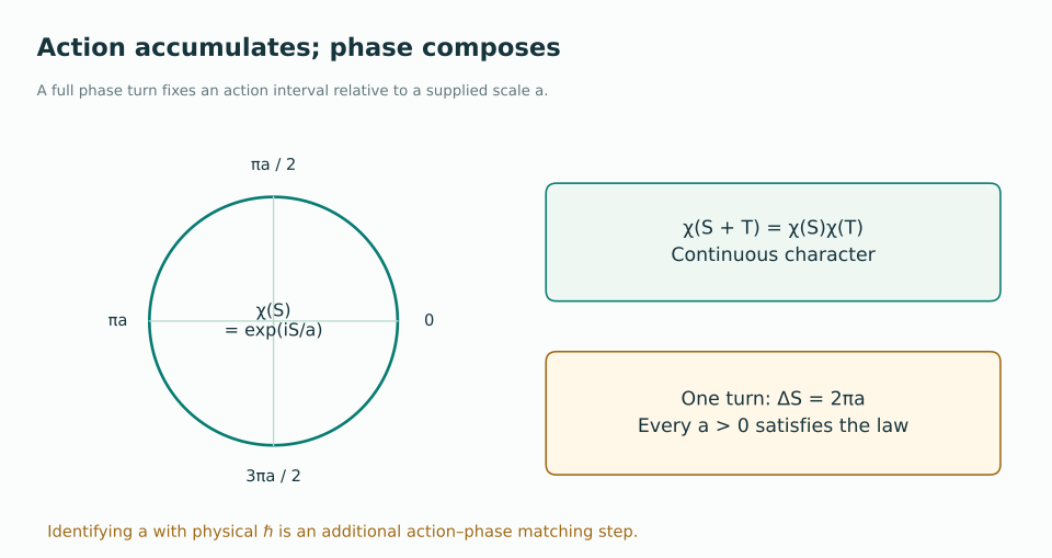
An action phase circle with one full turn equal to two pi times an arbitrary positive scale a — Figure ℏ1. Additivity fixes the functional form. The size of the action interval corresponding to a full turn is still a normalization choice. Download SVG

Match to physical quantum phases

If independently identified actions and observed quantum phases obey the bridge with a = ℏ, then h = 2πℏ and E = ℏω follow in the matched theory. A rest-state phase recurrence obeys T_C = 2πa/(mc²). Using a recurrence already computed from ℏ to “derive” ℏ would simply invert the same equation.

Compact phase and dual time are separate structures

The ordinary phase generator satisfies J² = −I. A split-complex bookkeeping unit used in some DTT formulations satisfies j² = +1. They have different algebraic properties. Compact inner recurrence can motivate a circle-valued phase, but a dynamical construction is needed to connect that phase to action. Neither the notation nor compactness supplies the missing numerical normalization.

What would strengthen this route?

Construct the additive physical action and its carrier from the same source dynamics; establish the continuous character rather than stipulating it; and obtain a dimensionless comparison with an independent physical standard. If only a discrete action lattice s₀ℤ is available, different phase slopes can be aliased, so the continuous-action assumption must be revisited.

Try the workbench

Change the action scale a and the sample action S. The displayed phase changes through S/a. Then inspect the comparison page: the same a also changes the mass and gravity dictionaries. This demonstrates shared scale dependence, not the independent selection of ℏ.

Source basis: C · §§3–4; pp. 5–7. These explanations summarize the stated models; they do not add a new physical selection theorem.

Explore ℏ.