


Assumptions, results and research status
Identifiability framework with synthetic, explicitly conditional examples
Assumptions
- A declared conventional baseline and a common list of atomic levels define every residual.
- Each proposed correction is generated by one operator family or an explicitly justified shared level-response map.
- Parameter dependencies and the covariance of measurements, constants, and theoretical terms are specified before assessing a residual.
Results
- A common level model automatically enforces δνₐ𝚌 = δνₐᵦ + δνᵦ𝚌.
- Contact corrections give fixed cross-transition ratios but can coincide with nuclear-size sensitivity.
- After whitening and projecting conventional-parameter directions, the remaining matrix rank identifies which proposed coefficients can be separately determined.
Open question: Which source-derived DTT operator produces a nonzero, parameter-restricted pattern that remains distinguishable after conventional atomic and nuclear response has been included?
1. Start with a distinguishable theoretical consequence
A residual is the difference between a defined observable and a defined reference calculation. It can arise from a missing conventional term, uncertain inputs, a mismatch of state labels, an experimental offset, or an additional physical contribution. Its smallness or unusual sign does not establish its origin.
A useful DTT proposal begins earlier, by deriving a restricted pattern across states. Paper 14’s strongest general contribution is its emphasis on shared shape functions and identifiability after conventional uncertainties are considered. [Paper 14, §§4–6 and 19] The theoretical work is to calculate the pattern and determine whether it is independent of the existing response directions.
This article therefore treats differential spectroscopy primarily as a problem in operators, linear algebra, and inference. The examples use exact fractions or synthetic coefficients. They do not contain fabricated measurements or claim a detected DTT anomaly.
2. Derive corrections to levels before correcting lines
Let the conventional Hamiltonian define states |a⟩ and energies Ea. A proposed small correction has the form δH = Σk ckOk, where the operators are specified and the coefficients have declared units and provenance. For an isolated nondegenerate level, first-order perturbation theory gives δEa = ⟨a|δH|a⟩.
Within a degenerate subspace, diagonalize the perturbation there first. Assigning diagonal expectation values in an arbitrary degenerate basis can miss mixing and give basis-dependent answers.
The bracketed differences form a response matrix X. Its columns are shared physical patterns. A freely adjustable correction for each line would replace this structure with an arbitrary vector and lose the predictive relation between states. The common-source aim of SMM/DTT is especially well expressed by a small set of source-derived operators controlling many such differences.
3. Transition networks enforce consistency
Assign a directed edge a → b to each signed interval. An incidence matrix T places −1 in column a and +1 in column b. Then the vector of transition corrections is TδE/h. Because the same state appears with the same energy on every edge,
For q connected levels, the space of stationary energy differences has rank q − 1. Adding the same constant to all levels changes no interval. A proposed level correction proportional to the identity is therefore invisible to these spectroscopy measurements.
Additional measurements of dependent intervals can still improve statistical precision or test systematic consistency. They do not create new theoretical sensitivity directions. For this reason, a long list of lines is not automatically an equally long list of independent tests.
The synthetic residual explorer calculates state shifts first and forms every interval from them. A cycle closes exactly for the model; numerical display rounding can create tiny apparent discrepancies, and real measurements have uncertainty around the corresponding identity.
4. Worked example: one contact coefficient
Take a first-order contact insertion with δEnS = K/n³ and zero leading shifts for states with ℓ > 0. This is a specified effective model with one energy coefficient K.
| Interval | hδν/K |
|---|---|
| 1S → 2S | −7/8 |
| 2S → 3S | −19/216 |
| 2S → 8D | −1/8 |
| 8D → 10D | 0 |
The ratio of the second shift to the first is 19/189. The 2S → 8D shift remains nonzero because the lower S state contributes. The final row is an energy interval; listing it does not assert that it is an allowed one-photon electric-dipole transition.
All intervals 2S → nD share the same leading contact correction. Subtracting two of them cancels the common lower-state contribution. This can isolate upper-state behaviour, but it also removes this particular signal.
A finite nuclear charge radius generates the same leading S-state n−3 dependence. Contact-pattern agreement alone therefore cannot identify a temporal origin.
5. A holonomy needs a physical energy map
A dimensionless phase or inverse-coupling residual ηa is not an energy. One possible model could supply a common map δEa = Kηa, with K derived independently. Another might justify state-dependent effective couplings. These are different hypotheses and should not be interchanged during comparison.
For the second case, suppose a model explicitly establishes αa = 1/(N + ηa) with N = 1/α. To first order, δαa = −α²ηa. Holding the other inputs fixed gives
This generally differs from multiplying ηb − ηa by an arbitrary transition frequency. If both η values are equal, their difference vanishes while the interval can still change through the common coupling. The level derivatives supply the missing physical information.
A source theory must justify such an effective coupling model or provide an alternative operator construction. Paper 14’s phase-based comparison ideas are used here with this explicit level-energy requirement. [Paper 14, sensitivity-map proposal]
6. Conventional parameters span competing response directions
Collect residuals into y. Near a declared reference, write y = Xc + Zδθ + ε. The columns of X describe the proposed source correction. The columns of Z describe changes in conventional parameters: for example a common energy scale, a nuclear radius, an unresolved field coefficient, or a shared theoretical remainder.
If a column of X lies in the span of Z, the selected observables cannot distinguish its coefficient from changes in those conventional parameters without additional information. This is an algebraic degeneracy, even if every frequency were known with very small uncertainty.
The contact example makes this concrete. If both a new effect and the only uncertain nuclear term shift nS levels by independent coefficients times n−3, their columns are proportional. Adding high-angular-momentum states, for which both leading effects vanish, does not by itself separate the two contact coefficients.
Independent nuclear information or a derived difference in radial, spin, or isotope dependence can break the degeneracy. Priors used for that purpose must be stated and justified; they are additional information in the result.
7. Whiten the covariance, then examine rank
Let C be the positive-definite covariance matrix of the residual vector, including the adopted measurement and theory uncertainties. Factor C = LLT and define whitened quantities ỹ = L−1y, X̃ = L−1X, and Z̃ = L−1Z. This rescales and decorrelates the observations according to their information content.
Let PZ be the ordinary orthogonal projector onto the column space of Z̃, computed by a numerically stable QR or singular-value decomposition. Then
The matrix X⊥ contains the proposed response that cannot be absorbed by unconstrained conventional changes. Full column rank is required to determine all proposed coefficients separately. A very small singular value signals a nearly degenerate combination with poor precision.
Numerical conditioning depends on the units assigned to coefficients, so compare singular values after choosing meaningful physical parameter scales. If C is singular because exactly dependent derived intervals were included, first remove redundancy or work in its supported subspace. Paper 14 develops the corresponding nuisance-projection viewpoint. [Paper 14, §19]
8. Choose complementary theoretical channels
The most useful added channel is one that changes the relation between candidate mechanisms. Higher angular momentum can suppress contact terms while retaining a genuinely longer-range perturbation. Fine-structure intervals can separate spin-dependent from spin-independent operators. Isotope changes can distinguish a universal electronic coefficient from a predicted nuclear scaling law.
These advantages are conditional on the proposed operator. A universal contact term does not become identifiable merely because a data set has an isotope label; freely uncertain isotope radii may still reproduce its shifts. A claimed angular-holonomy effect needs an angular matrix element, not just a new name for the same contact column.
Before considering a numerical residual, calculate the response matrix symbolically or in a converged source model. Inspect exact null directions, nearly parallel columns, and the effect of reasonable alternative baselines. This theoretical analysis identifies what information the programme actually lacks.
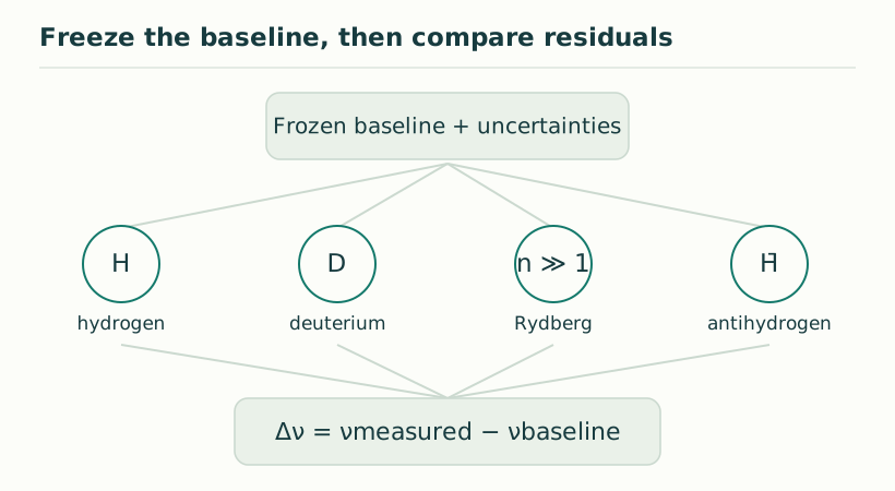
For readers exploring the idea, the residual explorer offers synthetic shared level corrections. Its role is to explain the geometry of a test; a physical DTT coefficient must come from the source calculation described in the research-status pages.
9. Define a meaningful outcome in advance
A successful calculation fixes a restricted operator family, derives or independently calibrates its coefficients, and predicts reserved level combinations. Agreement then concerns those specific consequences under the stated uncertainty model. A fitted coefficient is an estimate; it becomes an independent prediction only when transferred to observations not used to select it.
A null result is informative if the model predicted a nonzero effect with a specified scale. It is less restrictive if the coefficient was allowed to vanish freely. Similarly, failure to distinguish a source column from conventional response is an identifiability result, not evidence that either mechanism has been observed.
The collaboration priority is consequently precise: derive a shared source operator, calculate its state dependence, and establish a nonzero independent response direction. That work would strengthen the hydrogen programme even before any new measurement is considered.
Continue reading
Sources for this guide
Source manuscripts, version notes, and standard references are listed in the reference library.