
In this article
- A receiver dimension is only one ingredient
- Define the response and its source
- Derive the capacity formula
- Equal dimension, different capacities
- How capacity enters a spatial field
- What SMM/DTT must select next
Explain why the static response depends on the source and inverse response operator, not simply on the number of records. This is the central bridge required by the coupling proposal.
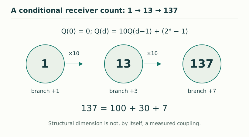
A static interaction depends on how a source excites a receiver and how costly each response direction is. Counting receiver modes gives neither of these pieces of information. This is the principal bridge between the structural value 137 and a possible physical coupling in the updated SMM/DTT draft.
Two apparatuses can have the same number of degrees of freedom yet different susceptibilities. Equally, differently sized apparatuses can have the same measured response. A theory of constants must therefore derive an appropriate response law, not only a state count. The draft expresses this issue in a finite-dimensional model that can be solved exactly.
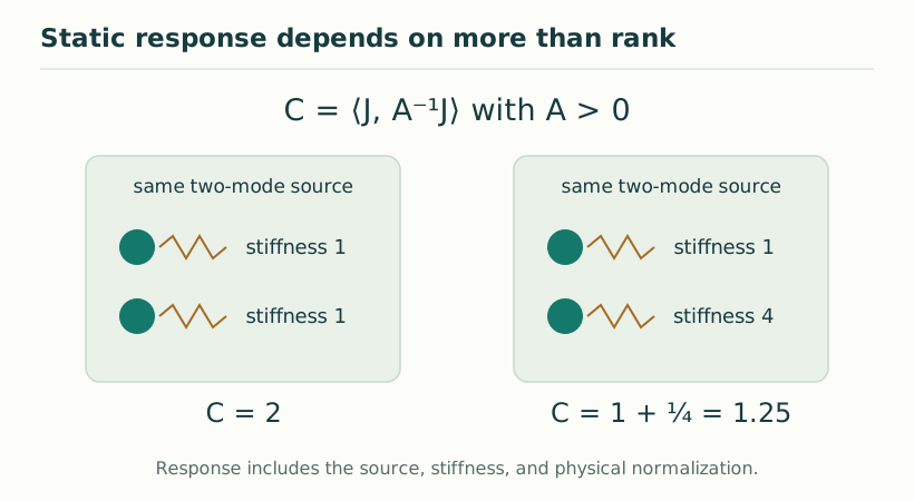
Let R be the complex receiver space and let F be a Hermitian response variable on it. The real inner product is ⟨X,Y⟩=Tr(XY). A positive self-adjoint operator A determines the quadratic energy, while a nonzero Hermitian source J determines the measured scalar current j=⟨J,F⟩.
The normalization of J is physical model data. Replacing J by a multiple changes the relation between the mathematical field and one unit of source. Likewise, A contains actual stiffnesses. A coordinate change that transports both objects preserves predictions; a change in one while holding the other fixed generally changes them.
Minimize the energy subject to a fixed scalar current j. A Lagrange multiplier gives AF=λJ, hence F=λA⁻¹J. Substituting into the constraint fixes λ=j/C, where C is the capacity defined above. The minimum energy is j²/(2C).
The same conclusion follows without multipliers by writing F=F*+Z with ⟨J,Z⟩=0. The cross term vanishes because AF* is proportional to J, and the remaining quadratic form in Z is positive. This also proves uniqueness. The observable response is therefore controlled by the source-weighted inverse stiffness, rather than the dimension of R by itself.
For isotropic stiffness A=κI and ordinary trace source J=I_N, the capacity is N/κ. This special class gives the inverse-rank energy factor 1/N. But the 137 receiver naturally contains sectors of dimensions 100, 30, and 7, so a source law could assign different positive stiffnesses to them while preserving their block symmetries.
With stiffnesses κ₁,κ₂,κ₃, ordinary trace coupling gives C=100/κ₁+30/κ₂+7/κ₃. Choosing κ₁=2κ and the others equal to κ produces C=87/κ, although the record count remains 137. This counterexample identifies the extra selection needed: common response coefficients do not follow merely from having a well-defined or covariant receiver.
On a fixed connected graph, impose a neutral source and a divergence constraint on edge currents. Minimizing the receiver variables on each edge reduces the problem to ordinary scalar current energy with coefficient 1/C. The graph Laplacian then determines the spatial Green function.
After an explicitly supplied three-dimensional continuum rescaling, the opposite-source potential has the form V(r)=−1/(4πCcont r). The dimensionless matter coupling is g=1/(4πacCcont), where a is the action scale and c the propagation speed. The continuum capacity has units inverse energy-length; it is not numerically identified with an unrescaled finite-graph coefficient.
A common-source explanation would compute A, J, the action-to-phase scale, and the propagation dictionary from the same source dynamics. It would explain why the receiver distinctions that enter the structural count also enter the field response with the required weights. That would turn a counting proposal into a dynamical mechanism.
Static measurements alone generally determine the capacity combination. They cannot uniquely reveal all internal modes or stiffnesses. Independent dynamical or sector-sensitive measurements would be needed to distinguish a genuine 137-mode construction from another model with the same capacity. This is a productive limitation: it states exactly what additional information a physical test must access.
KEEP THE CONNECTION
Scope of the argument. The capacity theorem is exact for the positive quadratic model; no physical electromagnetic source is selected by counting alone.
Draft file: smm_dtt_alpha0_137_v3.pdf
Working manuscript. Article-level references identify the consulted sections and the scope of the interpretation. No public URL was supplied for this exact manuscript version.
Source register →