
In this article
- The visible scalar can depend on hidden sectors
- Separate trace from traceless response
- Complete the square
- A two-sector numerical illustration
- Why static data do not identify every mode
- The connection to a conditional coupling
Introduce the reduction that gives capacity N/s under ordinary trace coupling. Show how hidden response sectors can affect an apparently simple scalar observable.
An experiment may couple only to the trace of a receiver field, yet the cheapest field configuration can move through traceless directions as well. Eliminating those unobserved directions changes the effective stiffness seen by the source. The Schur complement is the exact algebraic expression for this relaxation.
This provides a useful SMM/DTT distinction. A completed outer observable can be scalar even when the inner response has many coupled directions. The reduced scalar is calculated from the full dynamics; it is not obtained by assuming that every hidden direction is irrelevant. The model shows how hidden structure can affect a measurable interaction without being separately read out.
For a receiver of rank N, normalize the identity direction as e₀=I_N/√N. Every Hermitian field can be written F=xe₀+Z with Tr Z=0. Ordinary trace coupling fixes x=j/√N. In this orthogonal decomposition, write the positive response operator in block form with scalar entry u, cross-coupling b, and positive traceless block D.
Here u is a stiffness, not an elapsed time and not the action scale a. The vector b measures coupling between the trace channel and the traceless sector. If b vanishes, the visible direction is dynamically independent; if it does not, allowing Z to adjust lowers the energy at fixed j.
Expanding the quadratic form gives u x²+2x⟨b,Z⟩+⟨Z,DZ⟩. Add and subtract x²⟨b,D⁻¹b⟩ to rewrite it as a positive square plus a scalar term. The effective coefficient is s=u−⟨b,D⁻¹b⟩. Positivity of A guarantees s>0.
The minimizing hidden response is Z*=−xD⁻¹b. Substituting x=j/√N gives minimum energy s j²/(2N), so the capacity is N/s. This is exact and does not require the full response to be isotropic.
As a simple dimensionless illustration, take u=2, D=2 on one hidden direction, and b=1. The Schur complement is s=2−1/2=3/2. If the receiver rank is N, the source capacity is 2N/3. Ignoring the hidden adjustment would instead use N/2 and overestimate the energy required for the same current.
The positivity condition is visible here: the 2×2 response block has positive eigenvalues 1 and 3. If b were made so large that s≤0, the assumed positive energy model would fail. Thus the reduction both computes an effective response and checks stability. The example illustrates the algebra; it is not a fitted SMM/DTT parameter choice.
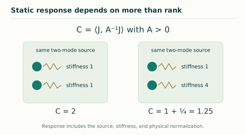
Two response models with the same N/s give the same source-dependent static minimum on a fixed graph. Changing N and s by the same factor leaves that capacity unchanged. Their internal fields, fluctuation spectra, and dynamics can still differ.
The result explains why a hydrogen-like Coulomb spectrum alone cannot verify the nested 100+30+7 receiver architecture. Such data constrain the effective potential coefficient. To probe the internal decomposition, one needs an independently fixed primitive stiffness or additional sources and frequencies sensitive to different response directions. A larger collection of static measurements of the same scalar combination does not automatically add that information.
After continuum matching, ordinary trace response gives g=scont/(4πacN). The structural value N=137 produces g=gprim/137, where gprim=scont/(4πac). The ideal proposal g=1/137 therefore requires gprim=1 as a separate normalization condition.
This is the precise point at which a deeper SMM/DTT source law would matter. It should calculate the trace coefficient after hidden sectors have relaxed and relate it to the same action and speed used by matter. Merely assigning equal names to these quantities does not establish the relation. The Schur reduction turns the missing derivation into an explicit, manageable target.
KEEP THE CONNECTION
Scope of the argument. Exact finite-dimensional response reduction; its physical source and continuum coefficients remain supplied interfaces.
Draft file: smm_dtt_alpha0_137_v3.pdf
Working manuscript. Article-level references identify the consulted sections and the scope of the interpretation. No public URL was supplied for this exact manuscript version.
Source register →