Concept maps, worked examples, and mathematical constructions from the article atlas. The captions identify conceptual schematics and idealized models; the curves are not experimental data.
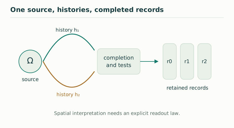
Figure 1. One source, histories, completed records. Conceptual reconstruction: composable source histories are tested and completed before a retained record becomes available. The source is not depicted as a point already located in space. View full size ↗
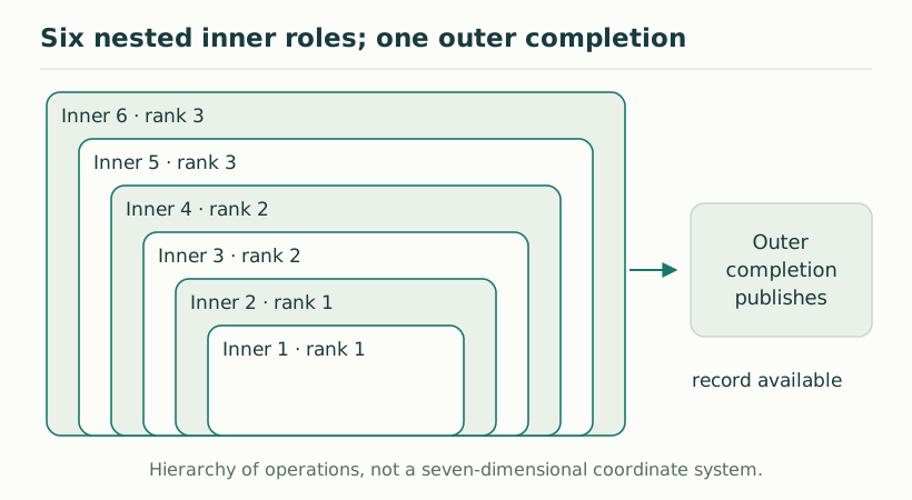
Figure 2. Six nested inner roles; one outer completion. The six inner roles are nested functional stages with readout ranks 1, 1, 2, 2, 3, 3. The outer completion publishes the resulting record. These are not seven independent time axes. View full size ↗
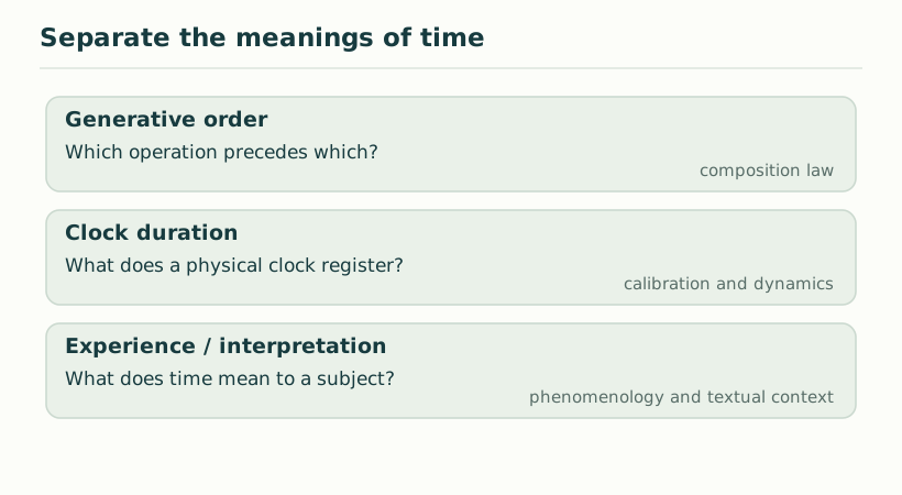
Figure 3. Separate the meanings of time. An interpretive map separates generative order, measured duration, and experienced or theological meanings. A relation between them is a question to formulate, not an automatic identification. View full size ↗
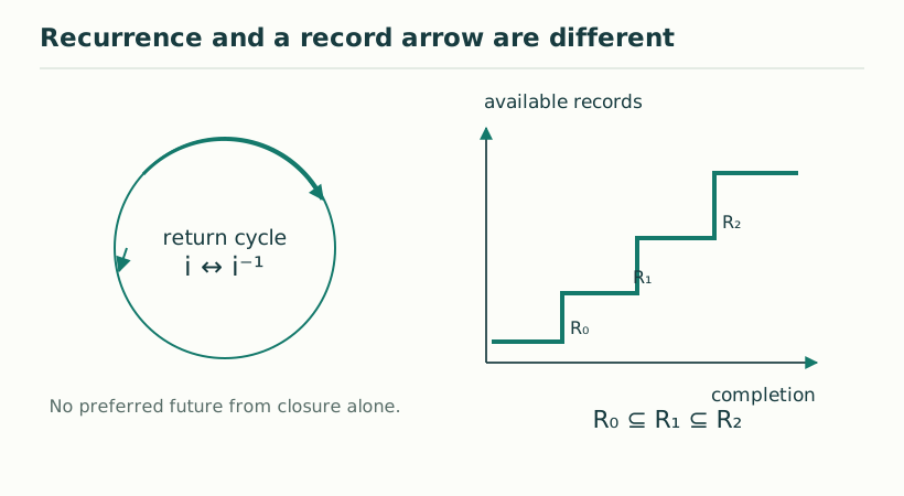
Figure 4. Recurrence and a record arrow are different. A reversible cycle admits both orientations. A record arrow requires an ordered availability relation, such as inclusion of retained records. Recurrence alone does not select a future. View full size ↗
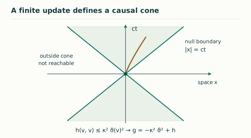
Figure 5. A finite update defines a causal cone. Illustrative finite-update geometry: displacement is bounded by update scale κ times projected inner duration. A Lorentzian metric or a shared light cone still requires the stated readout and field assumptions. View full size ↗
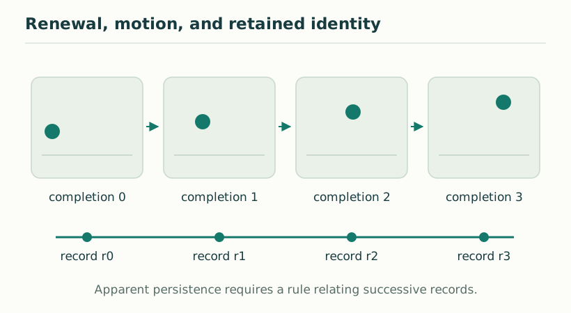
Figure 6. Renewal, motion, and retained identity. A film-frame analogy clarifies successive creation and apparent motion. It does not itself provide an update law, a conserved identity, or a continuum limit. View full size ↗
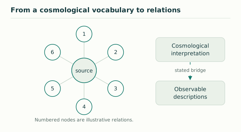
Figure 7. From a cosmological vocabulary to relations. The diagram is a reading aid for the SMM vocabulary: source, relations, manifested plurality, and observation. The arrangement does not assign physical locations to metaphysical terms. View full size ↗
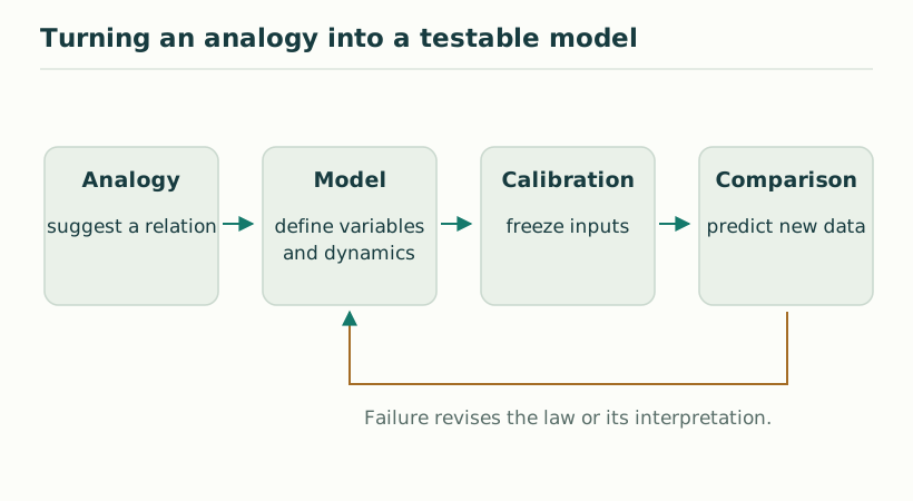
Figure 8. Turning an analogy into a testable model. A numerical or symbolic correspondence motivates a question. A physical claim needs a specified model, independent calibration, and a result that could disagree with observation. View full size ↗
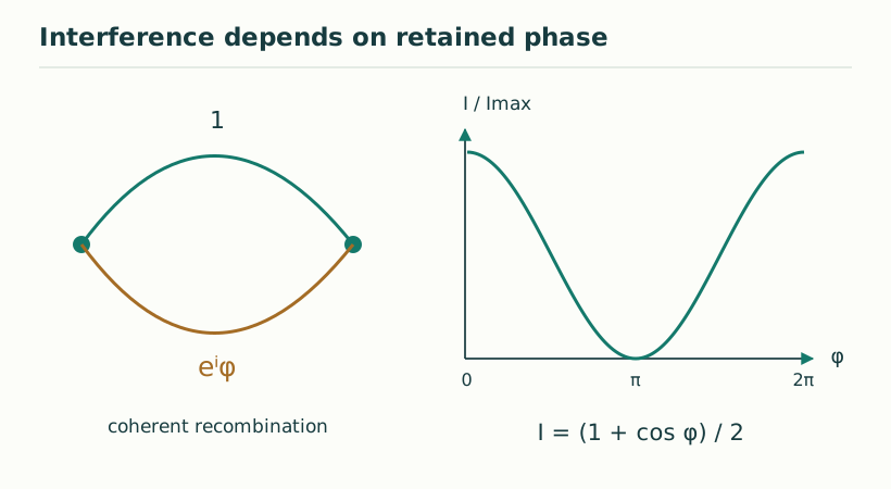
Figure 9. Interference depends on retained phase. The ideal two-path law I(φ) = |1 + eⁱφ|²/4 = (1 + cos φ)/2 is an illustrative quantum baseline. A temporal interpretation must specify which histories retain coherence and how the phase is controlled. View full size ↗
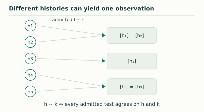
Figure 10. Different histories can yield one observation. The observational equivalence h ∼ k means that all admitted tests give the same result. Changing the test language can split an equivalence class and expose previously hidden distinctions. View full size ↗
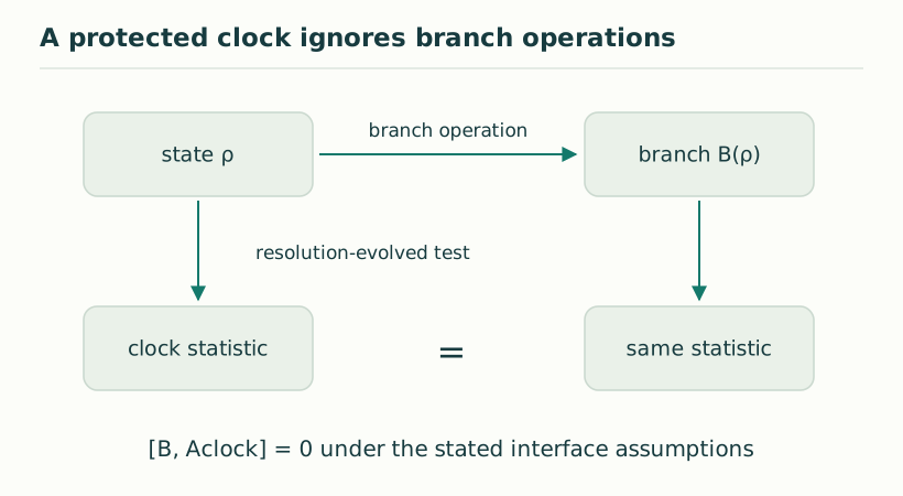
Figure 11. A protected clock ignores branch operations. In the stated stationary finite-dimensional model, branch invisibility is equivalent to the branch generator commuting with the resolution-evolved clock observable algebra. It is a criterion to verify, not an automatic law for every clock. View full size ↗
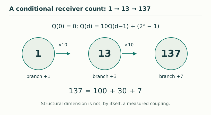
Figure 12. A conditional receiver count: 1 → 13 → 137. For the selected finite grammar Q(0) = 0 and Q(d) = 10Q(d−1) + (2ᵈ − 1), the depth-three output has 137 retained modes. Identifying 1/137 with an electromagnetic coupling needs additional response normalization and matching. View full size ↗
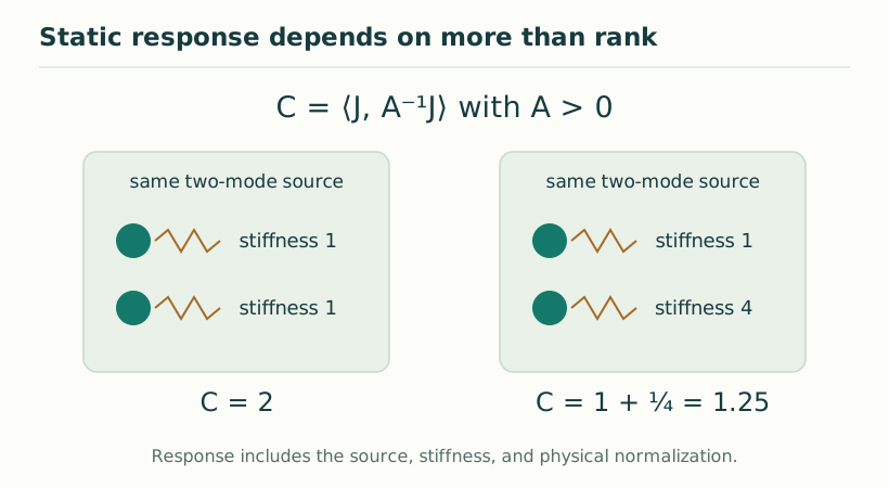
Figure 13. Static response depends on more than rank. With a positive response operator A and source J, capacity is C = ⟨J,A⁻¹J⟩. Equal dimensions can have different capacities; the displayed diagonal two-mode examples are exact illustrative arithmetic. View full size ↗
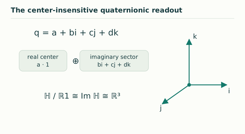
Figure 14. The center-insensitive quaternionic readout. Under the stated associative positive-norm and noncommutation hypotheses, the carrier is quaternionic. Quotienting the real center leaves the three-dimensional imaginary sector. This is a conditional readout result, not a standalone spatial dynamics. View full size ↗
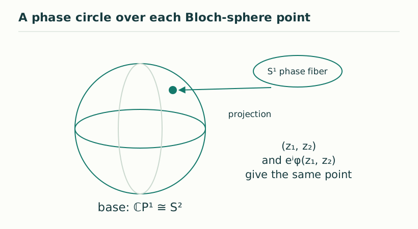
Figure 15. A phase circle over each Bloch-sphere point. For a normalized spinor (z₁,z₂), a common phase leaves the point of ℂP¹ ≅ S² unchanged. The Hopf bundle has total space S³; the drawing is a schematic of its fibers, not an embedding of S³ in ordinary three-space. View full size ↗
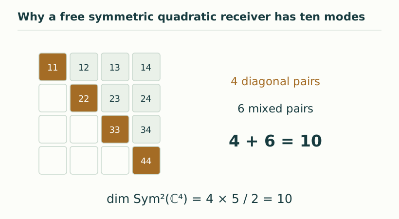
Figure 16. Why a free symmetric quadratic receiver has ten modes. A four-dimensional complex input has 4 diagonal quadratic modes and 6 unordered off-diagonal modes. Thus dim Sym²(ℂ⁴) = 4(4+1)/2 = 10. Selecting this receiver remains a model assumption. View full size ↗
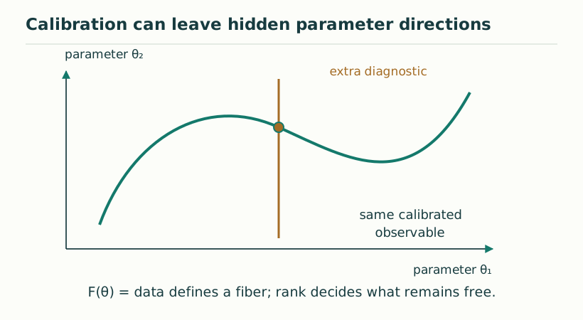
Figure 17. Calibration can leave hidden parameter directions. A fixed measurement may select a curve of models rather than one point. A genuine prediction must be constant on that calibration fiber, or require additional independently measured diagnostics. View full size ↗
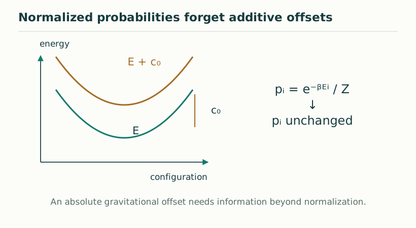
Figure 18. Normalized probabilities forget additive offsets. Adding an energy constant c₀ multiplies every Boltzmann weight by the same factor and leaves normalized probabilities unchanged. Such response alone cannot fix an absolute vacuum-energy offset. View full size ↗
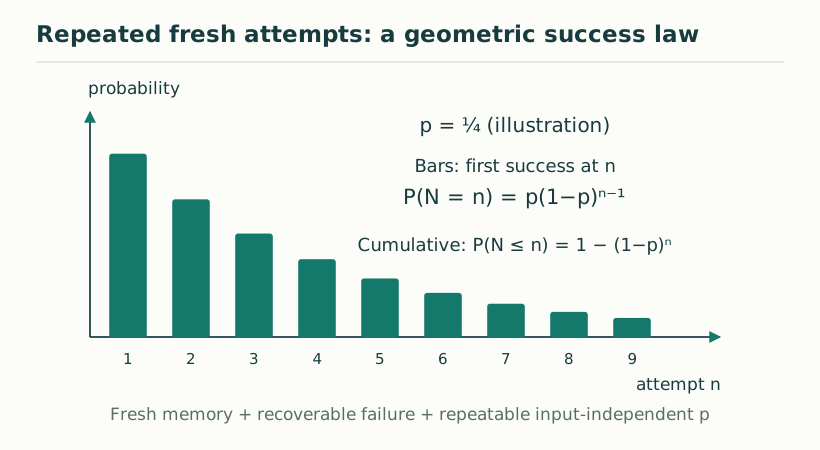
Figure 19. Repeated fresh attempts: a geometric success law. When a failed attempt restores the input and fresh attempts have the same independent success probability p, P(first success at n) = (1−p)ⁿ⁻¹p. The plotted example uses p = 0.25 and is not experimental data. View full size ↗
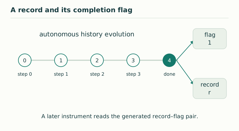
Figure 20. A record and its completion flag. A prescribed autonomous history dynamics can place a retained result and a flag in the same state. A later readout checks the flag and the result; assigning a flag by hand is not a dynamical construction. View full size ↗
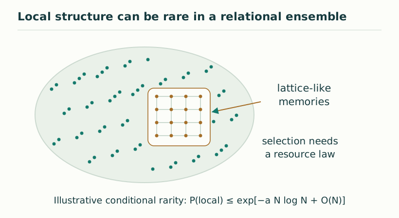
Figure 21. Local structure can be rare in a relational ensemble. A schematic ensemble contrasts arbitrary relational memories with a small lattice-like subset. In the stated permutation model, rarity is exponentially strong in N log N; constructing an example does not establish spontaneous selection. View full size ↗
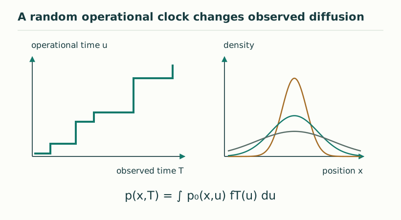
Figure 22. A random operational clock changes observed diffusion. The illustration subordinates diffusion in operational time u to an intermittent clock u(T). Flat portions represent waiting periods. The resulting memory does not imply two independently readable laboratory clocks. View full size ↗
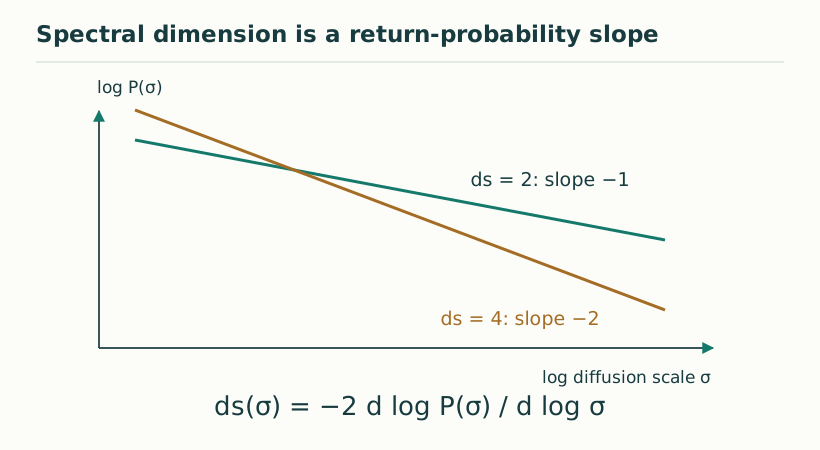
Figure 23. Spectral dimension is a return-probability slope. For the specified toy return law P(σ) = C σ⁻ᵈˢ/², the log–log slope is −ds/2. The two straight lines are ideal examples with ds = 2 and ds = 4; they are not observations of a dimensional flow. View full size ↗
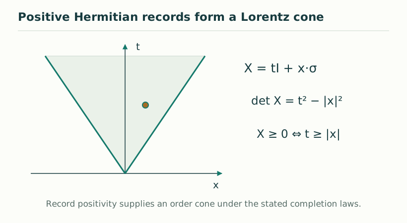
Figure 24. Positive Hermitian records form a Lorentz cone. Writing a Hermitian 2×2 record as X = tI + x·σ gives det X = t² − |x|². Positivity is equivalent to t ≥ |x|. The diagram is a two-dimensional section of the four-dimensional cone. View full size ↗
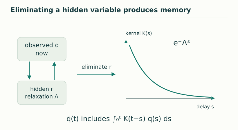
Figure 25. Eliminating a hidden variable produces memory. For a linear relaxing hidden sector, substitution produces a Volterra memory term. An exponentially decaying kernel is the simplest example; its fast limit can yield local effective dissipation under additional assumptions. View full size ↗
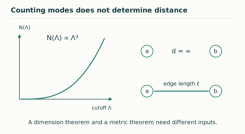
Figure 26. Counting modes does not determine distance. Spectral growth concerns how many modes lie below a cutoff. Distance concerns how observables vary under a normalized operator. The draft gives explicit examples in which the former is finite-dimensional while diagonal-state distances are infinite. View full size ↗
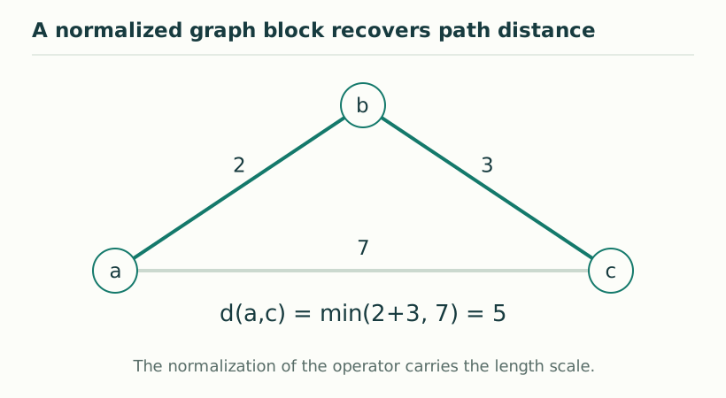
Figure 27. A normalized graph block recovers path distance. For the specified normalized spectral block, the distance equals weighted shortest-path distance. Here the illustrative route a–b–c has length 2+3 = 5, shorter than the direct edge of length 7. View full size ↗
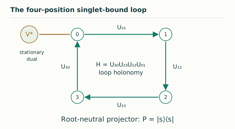
Figure 28. The four-position singlet-bound loop. A mobile carrier hops around four supplied positions while its stationary dual remains at the root. The root singlet penalty and the link holonomy determine the finite model response. This construction presupposes the lattice and carrier data. View full size ↗
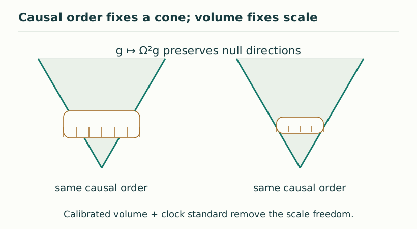
Figure 29. Causal order fixes a cone; volume fixes scale. A causal cone determines conformal geometry, while a calibrated volume law can fix the remaining scale. A physical interpretation as observer boosts requires the separate clock and detector covariance assumptions. View full size ↗
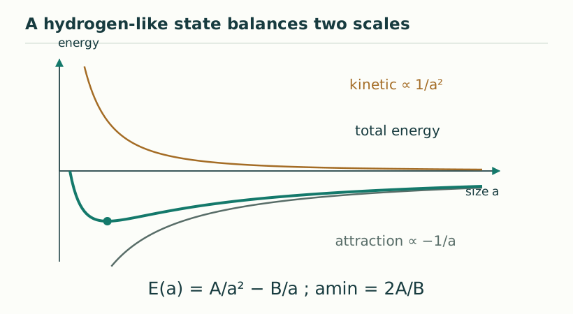
Figure 30. A hydrogen-like state balances two scales. The illustrative variational form E(a) = A/a² − B/a has a minimum at a = 2A/B for A,B > 0. Binding follows once kinetic and attractive terms are supplied; this calculation leaves B, and hence the coupling, free. View full size ↗
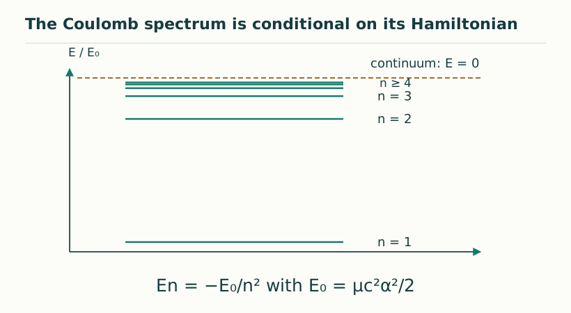
Figure 31. The Coulomb spectrum is conditional on its Hamiltonian. For the nonrelativistic Coulomb Hamiltonian, bound levels follow En = −E₀/n² and approach the continuum threshold. The diagram uses dimensionless E/E₀ and does not derive the coupling or supply radiative corrections. View full size ↗
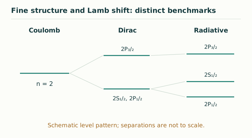
Figure 32. Fine structure and Lamb shift: distinct benchmarks. Schematic only, with deliberately exaggerated separations. For hydrogen n = 2, Dirac fine structure separates j = 1/2 from j = 3/2; radiative corrections further separate 2S₁/₂ and 2P₁/₂. No measured scale is plotted. View full size ↗
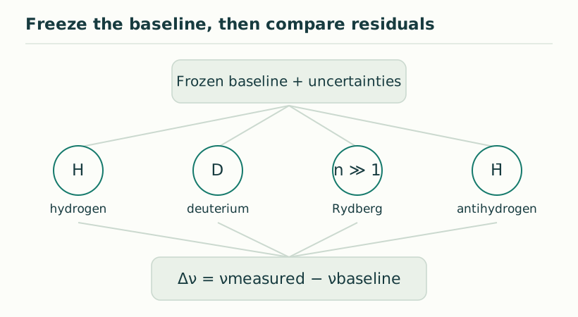
Figure 33. Freeze the baseline, then compare residuals. A differential test compares independently predicted and measured transitions across several systems. Shared nuisance effects can cancel only under a specified covariance model. The plotted markers are a design schematic, not data or DTT predictions. View full size ↗
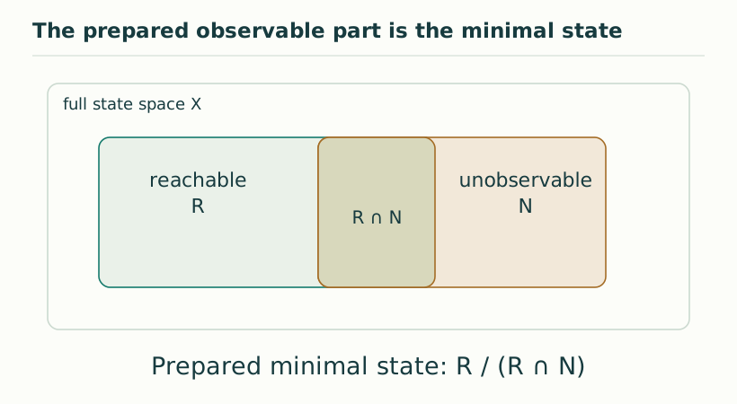
Figure 34. The prepared observable part is the minimal state. For a prepared linear interface, only reachable information that survives observational equivalence contributes to minimal behavior. The canonical state is R/(R∩N), not the entire hidden carrier. View full size ↗
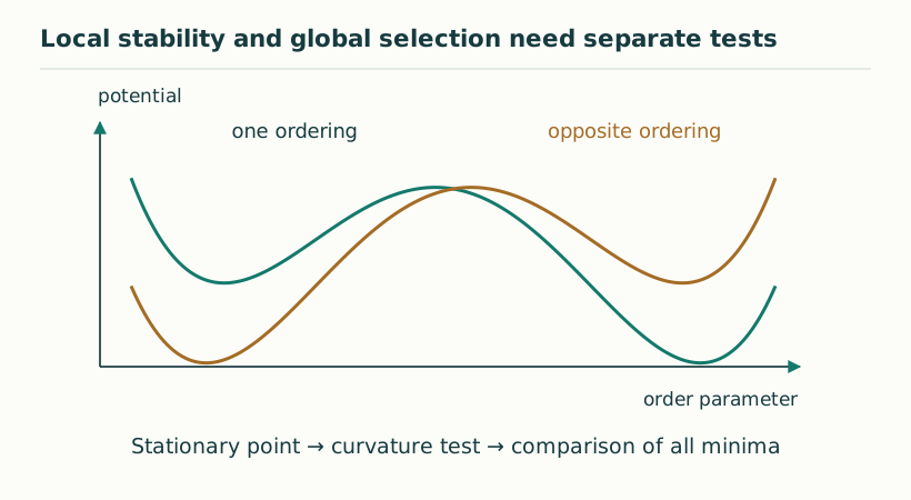
Figure 35. Local stability and global selection need separate tests. Illustrative order-parameter potentials distinguish a stable local well from the absolute minimum. The actual finite SU(2) threshold is obtained from the specified one-loop and deformation potential, not from this sketch. View full size ↗
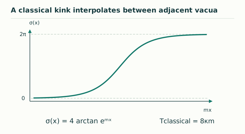
Figure 36. A classical kink interpolates between adjacent vacua. For the sine-Gordon-type dual-photon model, the classical profile σ(x) = 4 arctan exp(mx) interpolates from 0 to 2π and has Tclassical = 8κm under the stated normalization. Quantum gaps and matching remain separate questions. View full size ↗
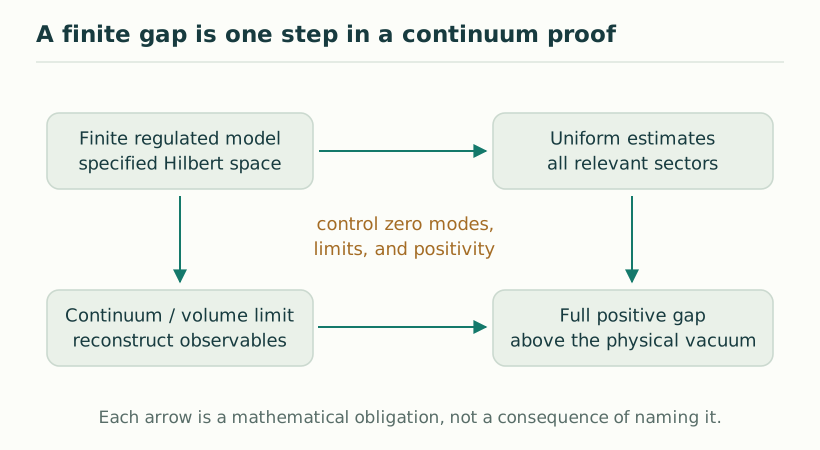
Figure 37. A finite gap is one step in a continuum proof. A finite-volume or charged-sector threshold does not by itself prove a full continuum mass gap. The diagram names distinct obligations: uniform control, physical-sector reconstruction, and a positive infinite-volume spectral threshold. View full size ↗
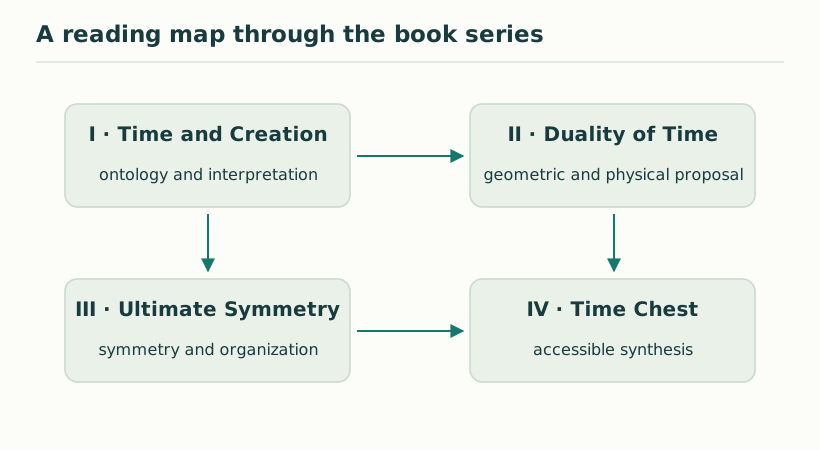
Figure 38. A reading map through the book series. A thematic map, not a claim that the later mathematical results follow automatically from the earlier texts. Readers can move from the ontology of time to physical constructions, then return to the interpretive questions. View full size ↗
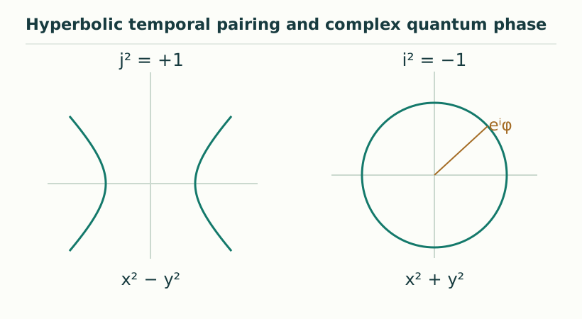
Figure 39. Hyperbolic temporal pairing and complex quantum phase. The split-complex unit j² = +1 supports a hyperbolic quadratic form. The ordinary complex unit i² = −1 supports circular phase rotations. A reconstruction must specify the bridge; the two units cannot simply be interchanged. View full size ↗
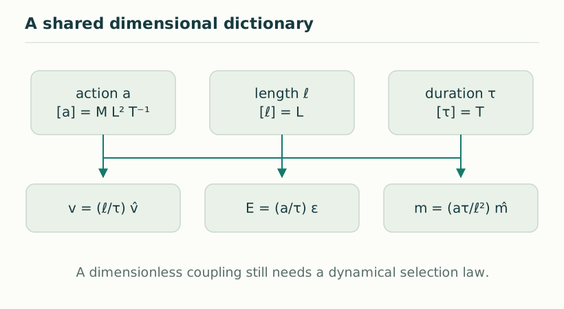
Figure 40. A shared dimensional dictionary. Dimensionless model outputs acquire physical units only after an action scale a, length scale ℓ, and time scale τ are supplied. These conversions are dimensional identities, not derivations of numerical constants. View full size ↗