Explain the distinction between effective delays caused by an irregular clock and a change in the vacuum limiting speed. Identify the observable quantities needed to tell these descriptions apart.
01A statistical realization of dual temporal roles
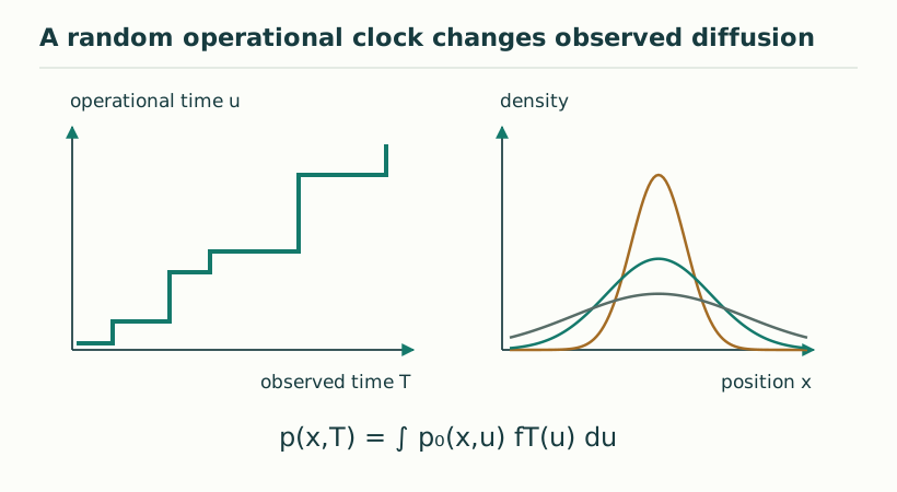
The renewal-clock model distinguishes microscopic events, operational time u accumulated through those events, and the outer duration T used to describe observations. Standard diffusion or unitary motion is specified in u. An irregular relation between u and T then changes the observed evolution. This is compatible with the DTT idea that generative progression and completed time need not coincide, but it is a particular stochastic realization, with a chosen waiting-time distribution and independence assumptions. It does not derive those choices from the single-source ontology or from the six nested inner stages. Those stages would need a separate mechanism explaining the observed event statistics.
02Delay can arise without changing microscopic propagation
Suppose a signal moves at a fixed operational speed v_u in the event clock u. If observed time T accumulates while the operational clock waits, the average distance covered per unit T can be smaller. The chain rule gives a projection factor χ=dE[u]/dT and an average effective speed v_eff=v_uχ in the stated ballistic approximation. This is a relation between two clocks. It does not automatically modify the local characteristic speed of the microscopic field equation.
χ(T)=dE[u(T)]/dT
v_eff(T)=v_uχ(T)
Figure 1. A random operational clock changes observed diffusion. The illustration subordinates diffusion in operational time u to an intermittent clock u(T). Flat portions represent waiting periods. The resulting memory does not imply two independently readable laboratory clocks. View full size ↗
03The anomalous-window calculation
Using E[u(T)]∼C_Dτ*^(1−D)Tᴰ gives χ(T)∼C_DDτ*^(1−D)T^(D−1). For D<1 this factor decreases through the pure heavy-tail window. The expression is asymptotic and cannot be extrapolated to arbitrarily small T or used as a universal cosmological clock. A realistic model may require a crossover back to ordinary timing. Individual arrival times also fluctuate around the mean, so the effective speed does not encode the whole propagation distribution.
χ(T)∼C_DD(τ*/T)^(1−D)
04A worked delay example
For D=1/2 and T=100τ*, the mean operational duration is approximately (2/π)10τ*=6.37τ*, and the local mean projection factor is approximately 0.0318. A ballistic process travels v_u times that mean operational duration. These large effects are deliberately illustrative. If the emitting process, detector and reference clock all experience the same time change, some apparent delay can cancel in dimensionless comparisons. An observable proposal must specify which clock is independent and which degrees of freedom share the intermittency.
05Avoiding a refractive-index shortcut
Material phase velocity, group velocity and signal-front velocity are distinct. Writing χ≈1/n may be a useful parametrization for one optical regime, but it is not a derivation of dispersion, absorption or causality from DTT. A proper comparison should predict the full frequency-dependent response and distinguish stochastic arrival-time broadening from deterministic dispersion and instrumental latency. The conceptual SMM/DTT contribution is the possibility that incomplete generative progress affects observed timing. Its empirical value would come from a specific clock-coupling law with signatures that survive these comparisons.
06A common random clock can hide in ratios
If both a propagating signal and a local oscillator evolve under exactly the same operational time u, the signal’s phase relative to that oscillator may remain unchanged even when both are slow relative to an external T. A measured delay therefore depends on which clock supplies the comparison. A useful model must distinguish a universal reparametrization from relative fluctuations between sectors. The latter can affect dimensionless timing ratios and be physically observable; the former may be largely conventional in a closed subsystem. This is especially relevant to SMM’s common-source proposal, where shared temporal structure should be specified before interpreting every slowing as a new propagation effect.
07What must be measured separately
The clock exponent D, the number of spatial coordinates, spectral dimension and a gravitational scaling dimension have different definitions. A random clock can change a diffusion diagnostic on a spatial manifold whose topology is unchanged. Similarly, an effective propagation delay is not automatically a change in a fundamental vacuum cone. A physical SMM/DTT application should identify a clock observable, state how its statistics are obtained, and compare the resulting predictions with a baseline using the same apparatus. Finite cutoffs, observation windows and normalization of probability kernels must be stated explicitly: their effects can be as important as the asymptotic power law.
Probability normalization is a practical consistency check throughout this programme. Integrating the clock density over operational time must give one at every observed time. Restoring a microscopic timescale inside a Laplace exponent can require a corresponding prefactor outside it; otherwise the averaged evolution will not preserve total probability. The same check should be made before calculating moments, return probabilities or quantum coherences. A fitted power law can look plausible even when a kernel is misnormalized, so explicit normalization is part of the derivation rather than a cosmetic convention.
KEEP THE CONNECTION
Key ideas
Clock intermittency can change effective durations while leaving operational dynamics unchanged.
Mean delay and arrival-time fluctuations are different observables.
A reference clock and a field-coupling prescription must be specified.
Scope of the argument. Effective clock-delay model; no general identification with refractive index or a changing fundamental vacuum speed.
Sources & further reading
smm_dtt_fractal_time_v3.pdf — working draftpp. 8–10, §6
Source editions and catalogue entries
Working manuscript
Fractal time — stochastic renewal-clock model, working draft v3
Draft file: smm_dtt_fractal_time_v3.pdf
Working manuscript. Article-level references identify the consulted sections and the scope of the interpretation. No public URL was supplied for this exact manuscript version.