A reading guide to the published temporal-asymmetry model. Organize its geometrical assumptions, reduction mechanism, and interpretation before comparing it with later working drafts.
The published temporal-asymmetry paper treats reversible and irreversible temporal roles using coupled connections and a projection to an observable description. Its central motivation is the coexistence of reversible microscopic laws with reduced evolution that remembers its history or relaxes. The two-parameter formulation in this paper should be read in its own terms; later same-cycle SMM/DTT drafts use a more restrictive organization.
The useful first question is operational: which data about the past must accompany a present observable to predict its future? A single clock parameter can coexist with memory. Conversely, adding a second formal parameter does not prove that an observer has acquired another independent clock.
02A solvable example of hidden memory
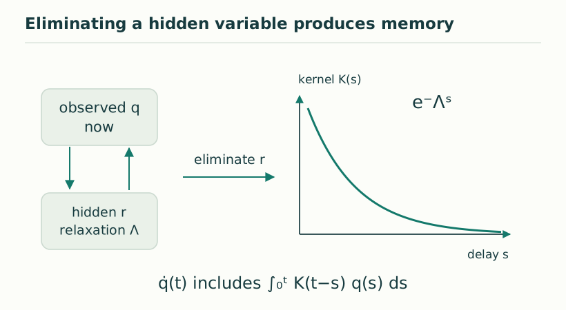
Let x be an observed variable and y an unobserved relaxation mode. Choose constants a, b, k, λ with λ>0 and the linear equations below. Solving the second equation by an integrating factor gives y(t) as a surviving initial contribution plus a weighted integral over earlier x. Substituting it into the first equation produces a memory term.
The calculation is exact for this supplied linear model. It shows why a local equation in a larger state space can become nonlocal in time after projection. Nothing has been fitted by declaring a kernel; the kernel follows from the eliminated mode and its coupling.
ẋ = -a x + b y, ẏ = -λ y + k x.
y(t) = e^(-λt)y(0) + k ∫₀ᵗ e^[-λ(t-s)]x(s) ds.
ẋ(t) = -a x(t) + b e^(-λt)y(0) + bk ∫₀ᵗ e^[-λ(t-s)]x(s) ds.
Figure 1. Eliminating a hidden variable produces memory. For a linear relaxing hidden sector, substitution produces a Volterra memory term. An exponentially decaying kernel is the simplest example; its fast limit can yield local effective dissipation under additional assumptions. View full size ↗
03A memory kernel is not automatically dissipation
The sign and strength of bk matter. Some choices produce stable relaxation; others can drive an instability. A monotonically decreasing energy or increasing entropy requires a suitable functional, positivity conditions, and control of the reversible part. The existence of an integral over the past does not establish any of these by itself.
If hidden relaxation is fast compared with the observed timescale, one may approximate y by kx/λ to leading order after initial transients. The reduced drift becomes (-a+bk/λ)x. This transparent example shows both the convenience and the limits of an adiabatic approximation: stability still depends on the supplied coefficients.
04Curvature records an ordering effect
For two covariant derivatives D₁=∂₁+A₁ and D₂=∂₂+A₂, their commutator contains F₁₂=∂₁A₂-∂₂A₁+[A₁,A₂]. A nonzero curvature means that transport around an infinitesimal loop can change the state. Operationally, performing two controlled procedures in opposite orders need not give the same result.
This can organize path dependence, but the order effect must survive the observation map to be measured. A curvature entirely inside an inaccessible sector may be mathematically nonzero and empirically invisible. The holonomy-localization articles make this distinction explicit.
[D₁,D₂] = F₁₂.
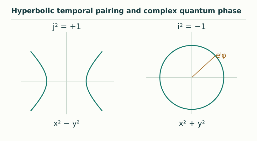
Figure 2. Hyperbolic temporal pairing and complex quantum phase. The split-complex unit j² = +1 supports a hyperbolic quadratic form. The ordinary complex unit i² = −1 supports circular phase rotations. A reconstruction must specify the bridge; the two units cannot simply be interchanged. View full size ↗
05Connecting the model to SMM and DTT
The conceptual connection is the separation between what the source does and what a completed observation retains. An observer may access x while the generative description carries both x and y. From the observer’s perspective, earlier values remain relevant because the present visible variable is not a complete state.
This is a concrete interpretation of temporal projection. It does not yet establish that the hidden variable is ontologically time rather than an unobserved degree of freedom. The stronger DTT claim would require a source-selection principle or observable restriction that cannot be removed by an equivalent one-time description.
06Reading the paper as a set of reusable tools
Follow three questions through the source: what are the independent temporal data, what is projected out, and which reduced invariants are retained? A connection can encode an order effect; an eliminated sector can generate a memory kernel; a positivity argument can establish a monotone functional. Those are distinct achievements and should be checked separately.
The practical bridge to the newer drafts is a controlled comparison of models. Translate their variables and interfaces before importing a result. A theorem proved for a two-parameter manifold cannot be treated as a theorem for a single recurrent action merely because both are described as dual-time.
KEEP THE CONNECTION
Key ideas
Eliminating a hidden mode gives an explicit memory kernel.
Path dependence, dissipation, and empirical detectability are distinct questions.
Different DTT formulations need an explicit translation before results are combined.
Scope of the argument. The linear calculation is an explanatory model; entropy production needs additional assumptions.
Journal metadata checked against the linked published text. The accompanying guide identifies the opening material consulted and develops explanatory examples; it is not an independent audit of every proof.