
In this article
- A calibrated model can still make predictions
- Define the calibration fiber
- The differential test and its limit
- The compact-phase example
- Detecting circular target reuse
- A concrete cross-sector protocol
Present the calibration-fiber criterion for a conditional prediction. An additional observable must be fixed across the allowed calibrated models to avoid merely reusing its target value.
Using measured data to determine a parameter is normal scientific practice. The important question is what remains fixed after that calibration. The draft formulates prediction as constancy across the family of all models compatible with the calibration data.
For SMM/DTT, this is a practical way to distinguish a promising conditional theory from numerical target reuse. A source model need not predict every constant without input. It should, however, produce additional consequences that cannot be independently retuned after calibration.
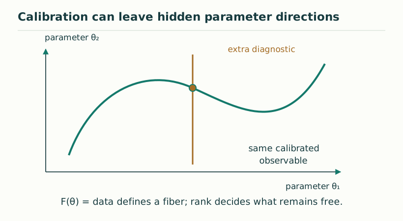
Let p collect the model’s free dimensionless inputs, C(p) the outputs used for calibration, and Ψ(p) a proposed new prediction. Fixing the observed calibration value selects the set of p satisfying C(p)=Cobs. This set is the calibration fiber.
If Ψ takes different values at different points of that fiber, calibration has not determined it uniquely. A prediction may then be a controlled range rather than a single number. If Ψ is constant on the admissible fiber, it is fixed by the calibrated model even when individual microscopic parameters remain unidentified.
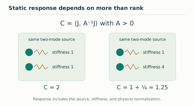
When C has constant rank, local parameter changes preserving calibration lie in the kernel of its derivative. The first-order ambiguity in Ψ vanishes exactly when dΨ annihilates every vector in that kernel.
This is only a first-order statement at one point. For example, Ψ(x)=x² has zero derivative at x=0 but is not constant nearby. If the derivative condition holds throughout a connected local fiber, integration along paths establishes constancy there. Controlled uncertainties, discrete model choices, and remote branches still need separate treatment.
The solvable compact response has a stiffness K(t) that is smooth and strictly decreasing. Once one adopts the response dictionary, a supplied coupling determines a unique t*. The exact same model then supplies its fourth-order response D₄(t*) and its comparator spectrum.
The fitted coupling is reconstructed input. The nonlinear response is a conditional output because no additional parameter was adjusted to it. To turn that output into a physical prediction, one must identify the measured source corresponding to the model’s phase perturbation and control the continuum and matter-matching errors. A calculated model observable is not automatically an experimentally accessible observable.
A dependency chain αref→t*→K(t*)→αreconstructed returns to the quantity used as its own calibration. It is a valid inversion calculation, but it does not derive α independently. Analogous loops arise when an electron clock is fixed from the electron mass or a geometric coefficient is fixed from Newton’s constant.
Not every mathematical cycle is illegitimate. Coupled equations and justified fixed-point problems can have genuine predictive solutions. Conversely, an acyclic diagram can still hide empirical choices. The useful audit asks which inputs were selected from data and whether the claimed test was among those inputs.
Choose an architecture before examining the intended test observable. Use one declared response to calibrate its remaining parameter, record the calibration uncertainty, and propagate that uncertainty through the exact model to a withheld nonlinear or spectral quantity. Compare the resulting interval with a measurement whose operator has been independently matched.
The conceptual SMM/DTT benefit is that a common source can connect sectors that would otherwise have independent parameters. A successful cross-sector relation is stronger evidence for that common source than repeatedly reproducing fitted constants. The same discipline should apply to the six nested-stage realization: nesting becomes explanatory when it restricts independently defined readouts, not when it only organizes a calculation after all values are supplied.
KEEP THE CONNECTION
Scope of the argument. Methodological criterion with a conditional compact-response example; experimental matching is still required.
Draft file: dtt_constants_reconstruction.pdf
Working manuscript. Article-level references identify the consulted sections and the scope of the interpretation. No public URL was supplied for this exact manuscript version.
Source register →