Use the draft’s qubit readouts to explain why very short observation windows can make clock calibration unstable. Precision depends on how distinguishable the tested responses are.
Two tests can distinguish every relevant direction in principle while doing so very poorly in the presence of noise. The clock draft makes this distinction explicit for a qubit. Any two nonparallel delayed readouts can give the desired exact commutant, yet a very short resolution window can make the inverse problem unstable.
This matters to SMM/DTT because a formal clock-selection theorem is not enough to demonstrate a physically reliable clock. The available temporal window, detector uncertainty, and preparation precision determine whether the mathematical distinctions can actually be resolved.
02The two delayed effects
Start with E+=(I+Z)/2 and resolution generator Kr=ℏωX/2. Use delays zero and θ/ω. The effects are F₁=(I+Z)/2 and F₂=(I+Z cos θ+Y sin θ)/2. For 0<θ<π their common Hermitian commutant is scalar.
Thus exact branch invisibility for both delayed tests forces a scalar branch generator in this qubit model. But the two effects become almost identical when θ is small and almost redundant again near π. Exact rank alone does not measure that near-dependence.
F₁=(I+Z)/2
F₂=(I+Z cos θ+Y sin θ)/2
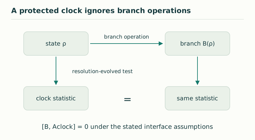
Figure 1. A protected clock ignores branch operations. In the stated stationary finite-dimensional model, branch invisibility is equivalent to the branch generator commuting with the resolution-evolved clock observable algebra. It is a criterion to verify, not an automatic law for every clock. View full size ↗
03Derive the conditioning constant
Represent a traceless Hermitian perturbation in the orthonormal Pauli basis. The squared commutator map has eigenvalues 2, 1+|cos θ|, and 1−|cos θ|. Its smallest singular value is therefore σ*=√(1−|cos θ|).
At a quarter period θ=π/2, σ*=1. For small positive θ, cos θ≈1−θ²/2 and σ*≈θ/√2. A response uncertainty divided by σ* is therefore amplified roughly as 1/θ. Shorter delay does not necessarily mean a more accurate calibration.
σ*=√(1−|cos θ|)
θ≪1 ⇒ σ*≈θ/√2
04A numerical illustration
At θ=0.1 radians, σ* is about 0.071, so the frame-dependent part of the error bound is roughly fourteen times larger than at θ=π/2. Both settings have the same exact scalar commutant. The difference is how much a hidden generator component can evade finite-precision measurement.
These values illustrate the exact formula rather than a proposed apparatus. A real design must include the uncertainty in θ and in the detector axes. If that uncertainty is comparable to the small angle separating the effects, a nominal singular value computed from the intended settings may not certify the true experiment.
05Bandwidth and conditioning solve different problems
A favorable σ* does not prevent a branch revival at the sampled excursion. Conversely, a bandwidth bound excluding revivals does not make nearly parallel effects informative. The finite theorem contains both σ* and sin[Wh/(2ℏ)] because each addresses a separate loss of identifiability.
The branch excursion h should lie within the independently justified bandwidth window, while the resolution delays should generate a well-conditioned effect frame. These two times are different protocol controls. Collapsing them into one generic “clock time” would obscure the design choices.
06Choosing an operating window
A practical calibration can compare candidate delay pairs by their smallest singular value, subject to coherence and hardware limits. Longer delays may improve angular separation but introduce dephasing, drift, or additional systematic errors. The useful choice maximizes information after those errors are included.
The theorem does not claim that the quarter-period pair is universally optimal once all resources are counted. It supplies an exact benchmark for the ideal qubit frame. A more complex clock requires its own finite commutator matrix and uncertainty analysis.
07The conceptual lesson for dual time
SMM/DTT distinguishes generative order from completed observation. This example shows that the ability to infer inner couplings from outer tests depends on the observation window itself. A hidden direction can be mathematically observable but practically inaccessible over a short window.
That observation should not be turned into a new fundamental uncertainty law without further derivation. It is an ordinary inverse-problem effect with an explicit coefficient. Its value for the research program is concrete: proposed clock independence can be accompanied by a stability estimate, rather than supported only by an exact idealized equality.
KEEP THE CONNECTION
Key ideas
Exact rank and robust calibration are different properties.
The qubit conditioning constant is √(1−|cos θ|).
Well-separated delayed effects improve certification, subject to hardware errors.
Scope of the argument. Exact qubit conditioning result within the specified readout model; not a universal time-resolution bound.
Sources & further reading
operational_clock_selection_focused.pdfWorking draft, pp. 6–9
Source editions and catalogue entries
Working manuscript
Operational Selection and Finite Calibration of Quantum Clocks
Working manuscript. Article-level references identify the consulted sections and the scope of the interpretation. No public URL was supplied for this exact manuscript version.