Use finite-dimensional examples to explain how reduced observations can appear irreversible. Keep the construction’s result separate from claims about the ultimate ontology of time.
The dual-time gauge draft distinguishes retained observable fields q from hidden generative variables r. Observation projects the larger state onto q, while couplings to r can still influence future observations. This is a concrete version of the SMM/DTT distinction between inner generation and outer realization. The mathematical reduction studied here starts from specified equations, coupling matrices and relaxation assumptions. It does not derive them from the six nested inner stages, nor identify those stages with independent time coordinates. The purpose is to show exactly how a chosen hidden sector can produce memory and, under stronger assumptions, monotone reduced dynamics.
02A two-variable model with explicit assumptions
Take one observed variable q and one hidden variable r with q̇=gr and ṙ=−λr−gkq, where λ,k>0. The structural functional is Ψ=kq²/2. This is an ordinary finite-dimensional model with hidden relaxation already included. It isolates a possible projection mechanism, but it is not itself a finite conservative universe. Any claim that the relaxation came from a larger conservative system would require that system and its bath or limiting procedure to be supplied.
q̇=gr, ṙ=−λr−gkq
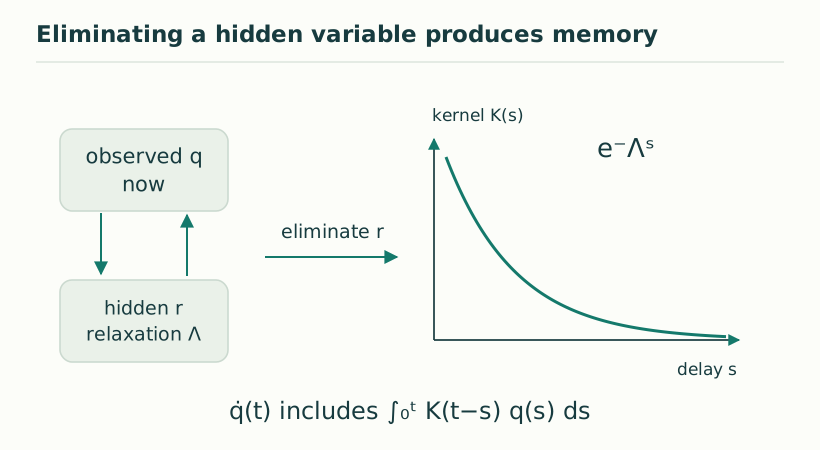
Figure 1. Eliminating a hidden variable produces memory. For a linear relaxing hidden sector, substitution produces a Volterra memory term. An exponentially decaying kernel is the simplest example; its fast limit can yield local effective dissipation under additional assumptions. View full size ↗
03The exact observable equation
Differentiate the first equation and use the second. The observable obeys q̈+λq̇+g²kq=0. Its characteristic exponents are [−λ±√(λ²−4g²k)]/2. With sufficiently large λ, there is a fast decaying mode and a slow mode approximately −g²k/λ. This slow rate agrees with the local realization metric M=g²/λ. The derivation gives a direct way to compare the exact two-variable dynamics with the adiabatically reduced law.
q̈+λq̇+g²kq=0
s_±=(−λ±√(λ²−4g²k))/2
04A worked comparison and an important limitation
Set g=k=1. For λ=10, the exponents are approximately −0.1010 and −9.8990, so the slow local approximation q̇≈−0.1q becomes accurate after the fast transient. For λ=1, the exponents are −1/2±i√3/2 and the motion oscillates while decaying. In that regime Ψ=q²/2 need not decrease at every instant: after crossing zero, q² increases again. Monotonicity of Ψ belongs to the stated local limit, not automatically to the exact memory equation.
05A larger dissipative quantity
For the exact toy system, E=(kq²+r²)/2 has derivative −λr²≤0. This distinguishes decay of the enlarged-system Lyapunov function from monotonicity of the observed part alone. It also makes clear where dissipation entered: λ was positive in the supplied hidden equation. In SMM/DTT the example is useful because it separates generation, projection and effective irreversibility with equations that can be checked. It does not establish the unique ontology of inner time, but it shows how to demand quantitative consistency before promoting a reduced arrow to a foundational claim.
E=(kq²+r²)/2, dE/dt=−λr²
06Hidden preparation controls the early observed motion
The exact second-order equation requires both q(0) and q̇(0), with q̇(0)=gr(0). A reduced first-order law retains only q(0), so it necessarily discards part of the preparation data. Its validity depends on the fast component becoming negligible. Two systems with the same initial visible q but opposite hidden r can initially move in opposite directions, even though both eventually approach the same equilibrium. This is a direct laboratory-style illustration of incomplete records. A DTT completion law should state whether it resets the hidden variable, retains it, or waits long enough that its effect is below a specified error tolerance.
07Interpretation of an irreversible reduced law
A reduced equation can lose predictive information because several larger states share one observed state. That does not make projection alone a universal source of thermodynamic entropy. Positive hidden relaxation, a chosen initial condition or reservoir, and a condition on the reversible flow do essential work in this model. The structural functional Ψ is not automatically Boltzmann, Gibbs or von Neumann entropy. Connecting its decay to a laboratory second law requires an operational coarse-graining, thermodynamic variables and calibrated coefficients. This qualification preserves the useful mechanism while preventing a model-level monotonicity theorem from being mistaken for an unconditional derivation of time’s arrow.
A finite closed Hamiltonian system preserves information globally and can display recurrences. Replacing some of its degrees of freedom by a permanently relaxing operator requires a specified approximation, reservoir or limiting regime. The exactness claimed for hidden-variable elimination is exactness relative to the supplied coupled equations, including their positive relaxation operator. It is not an independent proof that those equations follow from a conservative temporal action. A source-based derivation should track where the discarded information resides and over which interval the reduced dissipative description remains accurate.
KEEP THE CONNECTION
Key ideas
The exact toy model is a damped second-order system after elimination.
Observed Ψ can oscillate outside the fast-response regime.
Hidden relaxation is an explicit input, and the enlarged Lyapunov function is distinct.
Scope of the argument. Solvable dissipative toy model; it does not derive relaxation from a finite conservative source.
Sources & further reading
dual_time_entropy_v4.pdf — working draftpp. 21–25, §6.11; exact second-order and Lyapunov calculations developed here
Source editions and catalogue entries
Working manuscript
A Dual-Time Gauge Model for Projection-Induced Memory and Irreversibility
Draft file: dual_time_entropy_v4.pdf
Working manuscript. Article-level references identify the consulted sections and the scope of the interpretation. No public URL was supplied for this exact manuscript version.