Explain how removing the hidden sector produces an exact Volterra equation in the dual-time gauge model. A memory term can emerge even when the larger dynamics are specified locally in time.
The dual-time gauge draft distinguishes retained observable fields q from hidden generative variables r. Observation projects the larger state onto q, while couplings to r can still influence future observations. This is a concrete version of the SMM/DTT distinction between inner generation and outer realization. The mathematical reduction studied here starts from specified equations, coupling matrices and relaxation assumptions. It does not derive them from the six nested inner stages, nor identify those stages with independent time coordinates. The purpose is to show exactly how a chosen hidden sector can produce memory and, under stronger assumptions, monotone reduced dynamics.
02Start with coupled, time-local equations
Write the observable evolution as q̇=F(q)+Kr and the hidden evolution as ṙ=−Λr−Kᵀ∇Ψ(q). Here K couples retained and hidden variables, Λ is a stable hidden relaxation operator, and Ψ is the selected structural functional. Both equations depend on the present enlarged state. The observable q alone is generally insufficient because the same q can coexist with different hidden r. Eliminating r exposes that dependence rather than removing its physical effect.
q̇=F(q)+Kr
ṙ=−Λr−Kᵀ∇Ψ(q)
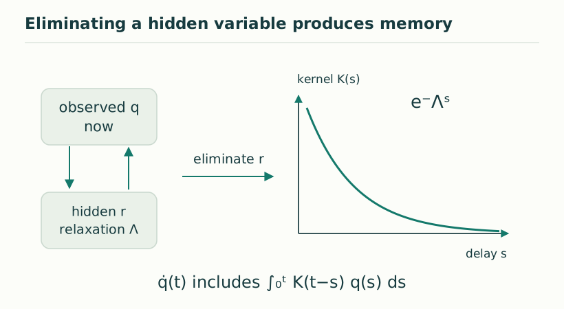
Figure 1. Eliminating a hidden variable produces memory. For a linear relaxing hidden sector, substitution produces a Volterra memory term. An exponentially decaying kernel is the simplest example; its fast limit can yield local effective dissipation under additional assumptions. View full size ↗
03Solve the hidden equation exactly
Variation of constants gives a freely decaying hidden initial state plus a convolution of the past observable gradient. Substituting into q̇ yields an exact Volterra equation. The memory kernel is K exp[−Λ(t−s)]Kᵀ, and the term K exp(−Λt)r₀ records the initially hidden preparation. It cannot be discarded before its decay is justified. No short-memory approximation is needed for this algebraic elimination.
r(t)=e^(−Λt)r₀−∫₀ᵗe^(−Λ(t−s))Kᵀ∇Ψ(q(s))ds
q̇=F(q)+Ke^(−Λt)r₀−∫₀ᵗKe^(−Λ(t−s))Kᵀ∇Ψ(q(s))ds
04A scalar worked example
For one observable and one hidden mode, let Ψ=kq²/2, K=g and Λ=λ>0. The memory term becomes −g²k∫₀ᵗe^(−λ(t−s))q(s)ds. Two preparations with the same q₀ but different r₀ have initial derivatives differing by gΔr₀. An experiment measuring only q₀ would therefore see apparently nonunique evolution unless it retains a history or specifies how r₀ was prepared. The exact kernel provides a systematic way to include that missing information.
05What the source interpretation contributes
DTT interprets r as a hidden generative sector and q as a completed readout. The elimination calculation itself is a standard dynamical mechanism and does not uniquely select that interpretation. Its value for the programme is diagnostic: a proposed completion map should say which variables disappear, which couplings survive, and which initial conditions remain relevant. A future autonomous source law could calculate K and Λ and thereby predict a specific memory response. Without that step, the article demonstrates a conditional mechanism rather than a unique temporal ontology.
06Memory is not the same as information flowing backward
The convolution integrates only over earlier times s≤t. Its nonlocality is temporal in the sense that a reduced state needs its past, not in the sense that later observations alter prior causes. A hidden initial state supplies another ordinary causal contribution. This distinction helps explain why eliminating variables can produce an equation that looks unfamiliar while remaining compatible with a well-posed enlarged initial-value problem. For DTT the physical question is whether the required hidden state is a generative completion variable, an ordinary environment, or an effective combination of both; the Volterra form alone does not decide that ontology.
07Interpretation of an irreversible reduced law
A reduced equation can lose predictive information because several larger states share one observed state. That does not make projection alone a universal source of thermodynamic entropy. Positive hidden relaxation, a chosen initial condition or reservoir, and a condition on the reversible flow do essential work in this model. The structural functional Ψ is not automatically Boltzmann, Gibbs or von Neumann entropy. Connecting its decay to a laboratory second law requires an operational coarse-graining, thermodynamic variables and calibrated coefficients. This qualification preserves the useful mechanism while preventing a model-level monotonicity theorem from being mistaken for an unconditional derivation of time’s arrow.
A finite closed Hamiltonian system preserves information globally and can display recurrences. Replacing some of its degrees of freedom by a permanently relaxing operator requires a specified approximation, reservoir or limiting regime. The exactness claimed for hidden-variable elimination is exactness relative to the supplied coupled equations, including their positive relaxation operator. It is not an independent proof that those equations follow from a conservative temporal action. A source-based derivation should track where the discarded information resides and over which interval the reduced dissipative description remains accurate.
KEEP THE CONNECTION
Key ideas
Exact elimination produces both a memory kernel and an initial-slip term.
A time-local enlarged model can be non-Markovian after reduction.
The source interpretation must specify hidden preparation and coupling.
Scope of the argument. Exact reduction of the stated linear hidden-sector equations; relaxation and coupling are supplied assumptions.
Sources & further reading
dual_time_entropy_v4.pdf — working draftpp. 16–19 and 21–23, §§6.6–6.11
Source editions and catalogue entries
Working manuscript
A Dual-Time Gauge Model for Projection-Induced Memory and Irreversibility
Draft file: dual_time_entropy_v4.pdf
Working manuscript. Article-level references identify the consulted sections and the scope of the interpretation. No public URL was supplied for this exact manuscript version.