Generating a neighborhood and preserving local transport
Separate reconstruction of spatial adjacency from the requirement that subsequent dynamics remain local. Explain the guarded transport rules used to preserve the generated metric.
SMM proposes that observable multiplicity can arise through one generative source. A mathematical realization must therefore distinguish the active source from retained memory: one cursor can visit many labels while the permutation tables and previous records remain available. Calling the cursor a monad does not eliminate that memory or derive its capacity. In this construction the labels initially carry no positions. A signed operation moves the cursor according to a permutation; a sequence of operations becomes a history, and tests decide which histories have the same completed record. Spatial adjacency is subsequently read from those completed transitions. This gives a precise route from operations to a candidate geometry, provided the chosen operation tables have suitable structure.
02Adjacency is only the first requirement
Suppose completed temporal operations have produced a graph of record labels. Calling neighbouring vertices close is meaningful only if physical updates respect that graph. An unrestricted later operation could exchange distant states in one step and destroy the relation between distance and causal influence. The draft therefore retains site identities, port identities and the joint quantum state. It restricts completed updates to on-site swaps followed by swaps across declared edges. The protection belongs to the allowed dynamics, not merely to the drawing of the graph.
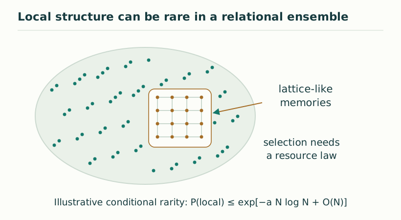
Figure 1. Local structure can be rare in a relational ensemble. A schematic ensemble contrasts arbitrary relational memories with a small lattice-like subset. In the stated permutation model, rarity is exponentially strong in N log N; constructing an example does not establish spontaneous selection. View full size ↗
03The support-growth proof
An on-site layer changes observables only within their current sites. An edge layer can enlarge support by at most one graph step. Applying this observation repeatedly proves an exact support bound after k completed episodes. Because each layer contains swaps on distinct ports, a serial implementation can reproduce the same completed operation without equating its private schedule with physical propagation. Unknown shared mobile memory would invalidate this simple argument if it carried information between remote sites.
support(Ψ*ᵏ(O_X)) ⊆ B_G(X,k)
S = E C, Ψ(ρ) = SρS†
04A transport example and its physical duration
Place a local observable at the centre of a chain. After one completed update its influence can reach adjacent sites; after two it can reach graph distance two. This is a cone in update depth. If each edge represents length ℓ and an independently calibrated completion takes Δt, its slope is at most ℓ/Δt in this simple circuit. A single cursor may need many primitive visits to execute that completion. For the nested finite-cube programme the manuscript counts 2q⁶ visits per episode, so bounded cursor speed prevents treating increasingly large archives as instantaneous.
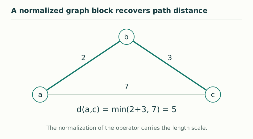
Figure 2. A normalized graph block recovers path distance. For the specified normalized spectral block, the distance equals weighted shortest-path distance. Here the illustrative route a–b–c has length 2+3 = 5, shorter than the direct edge of length 7. View full size ↗
05Continuous-time locality is a different estimate
A finite-range Hamiltonian with bounded total hopping strength yields exponentially suppressed propagation tails rather than the exact zero outside a circuit-depth cone. The paper proves a one-particle Dyson-series estimate by observing that reaching graph distance b requires at least b/r hops when each hop has range r. A many-body theory needs its own interaction assumptions and locality bound. Neither estimate selects a Lorentz-invariant speed or an Einstein equation. Their contribution is to identify the precise dynamical conditions under which completed geometry remains useful for predicting influence.
06The controller is a possible hidden communication channel
Suppose one unknown quantum register is carried by the cursor and interacts successively with distant sites. Even if the cursor’s schedule is private, the register can transfer information between those sites. The guarded-transport theorem excludes that possibility unless its induced coupling is separately bounded. A deterministic classical address controller that only selects predetermined disjoint gates has a different role. This distinction matters in a single-source ontology: saying that only one active source exists does not itself make completed propagation local. One must characterize what the source retains between visits and prove that its memory cannot implement unaccounted remote operations.
07What would complete the physical explanation
The six inner stages in this research programme are nested roles of a single generation–completion process. The seventh level publishes a completed configuration; it is not another independent time coordinate. The locality paper supplies concrete finite implementations of this architecture, but their schedules, memory and permitted transport remain specified inputs. A stronger SMM/DTT account would select those ingredients with one physical update law and explain why they persist under perturbation. It would also calibrate graph steps and completion counts against actual rulers and clocks. A proof about a finite labelled memory is valuable even before that programme is complete, provided its conclusion is kept at the level established by its hypotheses.
There is also a metric distinction inside the lattice example. Counting elementary signed operations produces a word metric, which on the standard lattice is the Manhattan metric. A Euclidean-looking embedding or cubic volume growth does not automatically replace that metric by an isotropic Euclidean norm. A continuum limit must specify the probe, its allowed directions and any averaging or refinement that makes its comparison law isotropic. This is why adjacency, volume growth, diffusion, calibrated distance and signal propagation should be checked separately even after an exact lattice neighbourhood theorem has been proved.
KEEP THE CONNECTION
Key ideas
Prepared adjacency must be preserved by allowed transport.
Circuit depth and laboratory time require separate calibration.
A private serial scan can transmit information unless its memory couplings are controlled.
Scope of the argument. Conditional circuit and one-particle propagation bounds; no universal relativistic locality theorem.
Sources & further reading
temporal_locality_v8(1).pdf — working draftpp. 21–24, Propositions 11.3–11.7 and Theorem 11.5
Source editions and catalogue entries
Working manuscript
Temporal locality — working draft v8
Draft file: temporal_locality_v8(1).pdf
Working manuscript. Article-level references identify the consulted sections and the scope of the interpretation. No public URL was supplied for this exact manuscript version.