Investigate information lost when a full generative state is reduced to spatial records. Explain why an apparently complete geometry may still be insufficient for autonomous prediction.
SMM proposes that observable multiplicity can arise through one generative source. A mathematical realization must therefore distinguish the active source from retained memory: one cursor can visit many labels while the permutation tables and previous records remain available. Calling the cursor a monad does not eliminate that memory or derive its capacity. In this construction the labels initially carry no positions. A signed operation moves the cursor according to a permutation; a sequence of operations becomes a history, and tests decide which histories have the same completed record. Spatial adjacency is subsequently read from those completed transitions. This gives a precise route from operations to a candidate geometry, provided the chosen operation tables have suitable structure.
02A spatial label can hide predictive information
A readout Q may assign several generative states to the same spatial site. If those states have different successors, their shared site label does not determine the next observation. The state then looks spatially complete but remains dynamically incomplete. This is a precise form of the DTT distinction between inner generation and outer presentation: what appears at a completed interface need not reveal every variable governing subsequent completion. Whether this loss is acceptable depends on the intended boundary and the future operations observers are allowed to test.
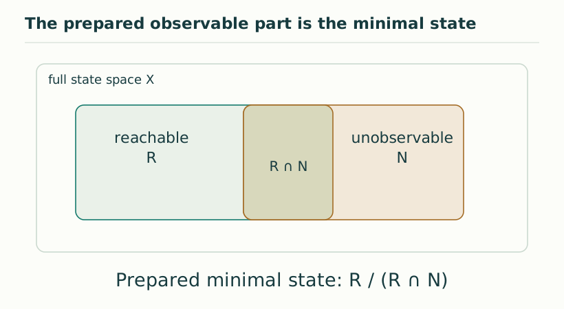
Figure 1. The prepared observable part is the minimal state. For a prepared linear interface, only reachable information that survives observational equivalence contributes to minimal behavior. The canonical state is R/(R∩N), not the entire hidden carrier. View full size ↗
03The nested-counter counterexample
In the six-digit radix-q construction, address zero has readout zero. Address q²−1 also has readout zero because its first paired digits both equal q−1. Their successors differ: zero advances the first digit, while q²−1 resets the first pair and advances the third digit. The next readouts are ℓe₁ and ℓe₂. Therefore no single map F on spatial sites can reproduce every elementary inner update. This conclusion is not a numerical approximation; it follows from two explicitly identical current readouts with distinct futures.
Q(0)=Q(q²−1)=0
Q(T0)=ℓe₁, Q(T(q²−1))=ℓe₂
there is no F with Q∘T = F∘Q for all inner addresses
04A general closure test
For a linear working state z, linear readout C and update M, a reduced evolution T satisfying CM=TC exists exactly when M preserves the kernel of C. To see necessity, two states differing by a vector in ker C have the same present readout; their difference after updating must still be unreadable. Conversely, kernel preservation makes T(Cz)=CMz independent of the representative. The smallest predictive quotient retains every direction that some future CMⁿ can detect. This criterion distinguishes a valid coarse-graining from merely deleting variables one would prefer not to track.
CM=TC ⇔ M(ker C)⊆ker C
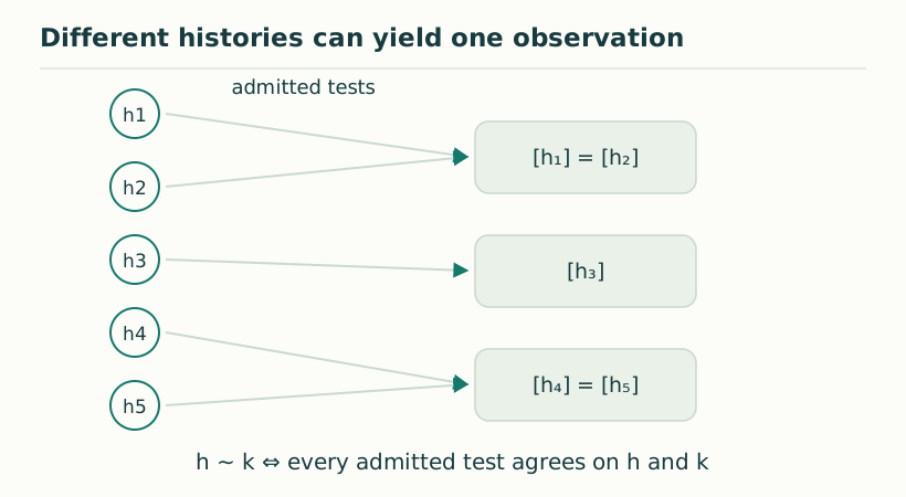
Figure 2. Different histories can yield one observation. The observational equivalence h ∼ k means that all admitted tests give the same result. Changing the test language can split an equivalence class and expose previously hidden distinctions. View full size ↗
05How outer completion can restore autonomy
At selected outer boundaries, the counter and sweep flag can return to prescribed values. The remaining state must still retain all port states and correlations that affect the next episode. A completion flag alone is insufficient. Measurements also change states, so their outcome records and instrument updates belong in the next predictive state. The research objective is to derive an economical completion rule whose retained variables are sufficient under the actual source dynamics. This is stronger than recovering a spatial image, and it turns the concept of completion into a concrete test of predictive adequacy.
06Memory can be added minimally
In the linear setting, the observable sequence C z, C Mz, C M²z and later values distinguishes precisely those state directions not lying in the intersection of all kernels ker(CMⁿ). Quotienting by that intersection gives a predictive state without retaining every microscopic coordinate. Thus the remedy is not automatically to make all hidden structure public. It is to retain enough information for the declared future tests. This offers a practical SMM/DTT design principle: choose a completion boundary, list admissible continuations, and calculate the minimal sufficient record before assigning it physical space or outer time.
07What would complete the physical explanation
The six inner stages in this research programme are nested roles of a single generation–completion process. The seventh level publishes a completed configuration; it is not another independent time coordinate. The locality paper supplies concrete finite implementations of this architecture, but their schedules, memory and permitted transport remain specified inputs. A stronger SMM/DTT account would select those ingredients with one physical update law and explain why they persist under perturbation. It would also calibrate graph steps and completion counts against actual rulers and clocks. A proof about a finite labelled memory is valuable even before that programme is complete, provided its conclusion is kept at the level established by its hypotheses.
There is also a metric distinction inside the lattice example. Counting elementary signed operations produces a word metric, which on the standard lattice is the Manhattan metric. A Euclidean-looking embedding or cubic volume growth does not automatically replace that metric by an isotropic Euclidean norm. A continuum limit must specify the probe, its allowed directions and any averaging or refinement that makes its comparison law isotropic. This is why adjacency, volume growth, diffusion, calibrated distance and signal propagation should be checked separately even after an exact lattice neighbourhood theorem has been proved.
KEEP THE CONNECTION
Key ideas
Equal spatial readouts can have different futures.
Autonomous reduction requires preservation of observational equivalence.
Outer boundaries can reset controller variables while retaining predictive physical memory.
Scope of the argument. Exact finite counterexample and linear closure criterion; no inference that all hidden variables must be observable.
Sources & further reading
temporal_locality_v8(1).pdf — working draftp. 21, Proposition 11.4; pp. 22–23, Theorem 11.5; linear criterion also in complexification_from_temporal_completion_v9.pdf p. 13
Source editions and catalogue entries
Working manuscript
Temporal locality — working draft v8
Draft file: temporal_locality_v8(1).pdf
Working manuscript. Article-level references identify the consulted sections and the scope of the interpretation. No public URL was supplied for this exact manuscript version.