A topic-led guide to the listed fractal-time preprint. Explain the distinction between a temporal mechanism, a dimensional diagnostic, and a complete spacetime reconstruction.
01What a temporal explanation of dimensional flow would mean
A dimension can count independent coordinates, describe the growth of volume, or characterize how a diffusion probe returns to its starting point. A temporal model can alter the third quantity without changing the first. This distinction is central when reading the fractal-time proposal and its newer renewal-clock formulation.
The SMM/DTT connection is that observed elapsed time need not parameterize microscopic updates uniformly. If the clock relating source activity to completed records is irregular, a probe described against observed time can display anomalous scaling even on a fixed spatial graph.
02Two clocks in a statistical construction
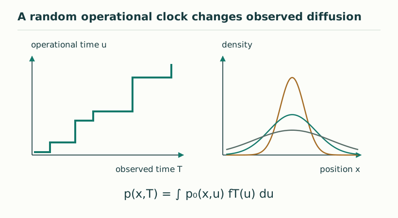
Let u count operational progress and t be the time assigned to observation. A random nondecreasing process E(t) can connect them. If Y(u) is an ordinary diffusion, X(t)=Y(E(t)) is the same underlying spatial motion sampled through the random clock.
The probability density of X is an average of the operational kernel over the distribution of E(t). This averaging is called subordination in the broad clock-change sense; inverse-subordinator constructions must be distinguished from direct subordinators because their equations and scaling properties differ. The distribution and independence assumptions are part of the model.
P(x,t) = ∫₀∞ K(x,u) f(u,t) du.
Figure 1. A random operational clock changes observed diffusion. The illustration subordinates diffusion in operational time u to an intermittent clock u(T). Flat portions represent waiting periods. The resulting memory does not imply two independently readable laboratory clocks. View full size ↗
03How a power-law return diagnostic is computed
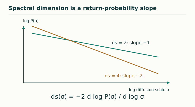
Suppose an admissible return observable obeys P₀(t)=C t^(-q) over a specified interval. Its scale-local spectral dimension is d_s(t)=-2 d logP₀/d logt=2q there. This is a calculation on a chosen diagnostic, not a count of coordinates.
For ordinary Euclidean diffusion in d dimensions, the return density has exponent d/2. Replacing operational time by a deterministic u=t^D would formally give exponent Dd/2. Random clocks cannot always be substituted this way: averaging a singular kernel over a distribution is a separate operation with its own convergence requirements.
d_s(t) = -2 d log P₀(t) / d log t.
04The finiteness condition matters
For an inverse-stable clock, small operational times can contribute strongly to the average of u^(-d/2). In dimensions at least two, the coincident continuum heat kernel may diverge under the relevant small-u behavior. A formal scaling argument that silently assumes a finite value at the origin can therefore fail.
A finite spatial regulator, a smeared return observable, or a carefully identified asymptotic regime can produce meaningful diagnostics. One should state which is used and analyze its cutoff dependence. The appropriate result is then about that well-defined observable; it need not be the unqualified identity d_s=Dd for every inverse-stable process.
Figure 2. Spectral dimension is a return-probability slope. For the specified toy return law P(σ) = C σ⁻ᵈˢ/², the log–log slope is −ds/2. The two straight lines are ideal examples with ds = 2 and ds = 4; they are not observations of a dimensional flow. View full size ↗
05What can be learned from a finite graph
On a finite graph, the operational return probability is bounded and the clock average is well-defined under a normalized waiting-time law. At sufficiently long times it approaches a stationary value, so the local spectral dimension tends toward zero rather than remaining at an intermediate power-law value forever.
A useful numerical study therefore plots several scales and graph sizes. An intermediate slope can support a scaling regime, but early-time resolution effects and late-time finite-size saturation must be identified. This is a more informative experiment than selecting one fitted exponent from one small graph.
06The conceptual gain for DTT
The model makes a precise point: temporal statistics can change what an observer infers from a propagation or diffusion experiment. It does not by itself generate three-dimensional space, establish quantum gravity, or identify the random clock with the unique Single Monad dynamics. Those require additional structure.
The research opportunity is to derive the waiting-time law and its regime from a specified source, then compare several diagnostics fixed by that same law. Return probabilities, relaxation kernels, and clock fluctuations could become related outputs. Their agreement would be more constraining than a chosen dimensional-flow curve alone.
KEEP THE CONNECTION
Key ideas
Spectral dimension is a probe-dependent scaling diagnostic.
A random clock requires an average, not a simple substitution of time variables.
Finite return probabilities and regulator control are essential.
Scope of the argument. The elementary return-law calculation is exact when its observable exists; universal dimensional-flow claims require further hypotheses.
Bibliographic status is as listed on the author’s papers page, checked 16 October 2026. The accompanying thematic guide states its source coverage and the additional steps needed to assess the proposed results. A direct destination could not be resolved; the link opens the papers catalogue where the title can be located.