Three-frequency counting and inner spectral dimension
Introduce the cubic eigenvalue-counting result for the inner operator. Explain why including the separate outer circle changes the count in the compact auxiliary model.
The spectral-triple draft translates recurrent generative operations into shifts, frequency operators and spectra, while completed records are intended to support empirical ordering and distance. This is a mathematical interface for SMM/DTT rather than a complete source dynamics. Its three paired frequency labels represent a specified inner spectral sector. They must not be confused with six independently variable temporal coordinates: the six inner stages of the conceptual programme are nested generative roles, and outer completion is their record interface. A derivation still has to show why this particular operator representation is selected and how its records become physical displacements.
02Why one clock does not supply cubic growth
For D₁=ωN on ℓ²(ℤ), the number of absolute eigenvalues no greater than Λ is 2 floor(Λ/ω)+1. It grows linearly, so this frequency model has counting dimension one. A picture of a clock winding through three directions cannot replace that spectral calculation. Cubic growth requires additional mode labels or a specified degeneracy law whose cumulative count has the required power.
N₁(Λ)=2⌊Λ/ω⌋+1
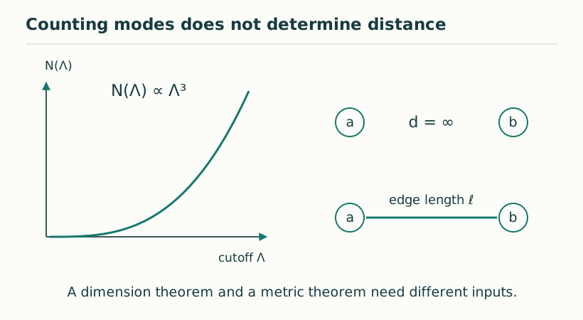
Figure 1. Counting modes does not determine distance. Spectral growth concerns how many modes lie below a cutoff. Distance concerns how observables vary under a normalized operator. The draft gives explicit examples in which the former is finite-dimensional while diagonal-state distances are infinite. View full size ↗
03Counting three paired frequencies
The model takes n∈ℤ³ and D_in=Σ_aΓ_aω_an_a, with anticommuting Hermitian Clifford matrices. Squaring cancels cross terms and gives Σ_aω_a²n_a² times the identity. Counting |D_in|≤Λ therefore amounts to counting integer lattice points in an ellipsoid. Its leading volume is 4πΛ³/(3ω₁ω₂ω₃), multiplied by the finite internal multiplicity. The exponent is three even when the positive weights are anisotropic.
D_in²=(ω₁²n₁²+ω₂²n₂²+ω₃²n₃²)I
N_in(Λ)∼m_fin 4πΛ³/(3ω₁ω₂ω₃)
04An anisotropic example
Choose weights (1,2,4). The frequency ellipsoid has semiaxes Λ, Λ/2 and Λ/4, so its volume is one eighth of the equal-weight case. Its growth exponent remains three. Thus the counting dimension does not establish isotropic physical rulers: anisotropy changes coefficients while preserving the exponent. A separate readout law must identify whether these weights correspond to physical directional scales, internal normalization or a regulator choice.
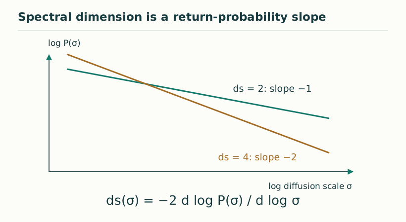
Figure 2. Spectral dimension is a return-probability slope. For the specified toy return law P(σ) = C σ⁻ᵈˢ/², the log–log slope is −ds/2. The two straight lines are ideal examples with ds = 2 and ds = 4; they are not observations of a dimensional flow. View full size ↗
05What adding the outer circle changes
If the auxiliary operator also includes an independent outer Fourier label p, its full compact counting problem has four growing integer directions. The three-dimensional claim applies to the inner operator, a fixed outer mode or a trace-per-unit-time reduction. This bookkeeping matters for DTT because outer completion and inner generation have different interpretive roles. The proof is a conditional Weyl-law calculation for three supplied pairs; it does not select three pairs from source unity, derive graph distance, or prove that the resulting spectral sector is the spatial manifold of the observed world.
06Bounded corrections preserve a leading exponent, not every observable
Adding a bounded finite matrix shifts high-frequency eigenvalues by a bounded amount, so it does not change the leading cubic count. A bounded hopping perturbation can simultaneously make a major difference to localized metric behaviour. This illustrates why robustness of a spectral dimension is weaker than robustness of all geometry. In an SMM/DTT model, one should report which perturbations preserve counting, which preserve finite distances and which preserve the operational cone. A common exponent across several regulators is encouraging, but does not show that the source uniquely selected the same physical geometry in each realization.
07Three diagnostics with different jobs
Spectral counting measures how the number of modes grows with frequency. A commutator seminorm measures which observables can vary between states while remaining Lipschitz bounded. An operational calibration connects these mathematical states and scales to actual records, distances and clocks. None of the three substitutes for the others. A compact auxiliary operator can have a clear counting exponent and nevertheless give infinite distances between selected localized states. Likewise a finite graph can have an exact distance without proving a smooth manifold limit or Lorentzian dynamics. Keeping these tests separate makes the reconstruction more informative and prevents a numerical plateau from being mistaken for complete spatial emergence.
Operator normalization is physical data once a spectral construction is used for measurement. Replacing D by aD multiplies its eigenvalues by a but divides its Connes distances by |a|. The counting exponent can remain unchanged while all calibrated lengths change. Likewise a bounded finite multiplicity changes a leading counting coefficient without changing its exponent. A proposed temporal explanation of geometry should therefore state both dimensionless structural results and dimensional calibrations. Agreement of an exponent with three is useful, but it cannot fix a ruler, a clock or their conversion by itself.
KEEP THE CONNECTION
Key ideas
One frequency label gives linear counting growth.
Three supplied paired modes yield cubic growth even with unequal weights.
The full compact product including outer frequency is a different count.
Scope of the argument. Conditional spectral dimension of the stated operator; spatial dimension and isotropy require separate reconstruction.
Sources & further reading
dual_temporal_spectral_triples_v3.pdf — working draftpp. 10–14, §§6–7, Proposition 7.1 and Theorem 7.2
Source editions and catalogue entries
Working manuscript
Complex-Time Spectral Triples and the Separation of Spectral Dimension from Metric Distance
Draft file: dual_temporal_spectral_triples_v3.pdf
Working manuscript. Article-level references identify the consulted sections and the scope of the interpretation. No public URL was supplied for this exact manuscript version.