Introduce the graph-block construction whose Connes distance equals weighted shortest-path distance. Explain the normalization assumptions behind that equality.
The spectral-triple draft translates recurrent generative operations into shifts, frequency operators and spectra, while completed records are intended to support empirical ordering and distance. This is a mathematical interface for SMM/DTT rather than a complete source dynamics. Its three paired frequency labels represent a specified inner spectral sector. They must not be confused with six independently variable temporal coordinates: the six inner stages of the conceptual programme are nested generative roles, and outer completion is their record interface. A derivation still has to show why this particular operator representation is selected and how its records become physical displacements.
02The normalized edge construction
For each undirected edge e={x,y} of a finite connected graph, choose a positive length ℓ_e. Represent a vertex function f by diag(f(x),f(y)) on that edge, and set D_e to the off-diagonal matrix with entries 1/ℓ_e. Take the direct sum over edges. This particular direct-sum normalization makes the commutator norm the maximum edge slope. A generic adjacency matrix does not automatically have the same norm or exact distance formula.
D_e=ℓ_e⁻¹ [[0,1],[1,0]]
L_D(f)=max_e |f(x)−f(y)|/ℓ_e
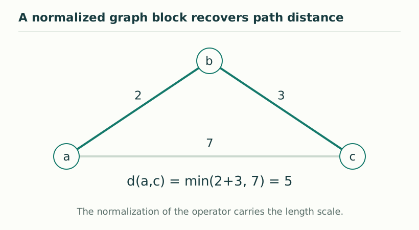
Figure 1. A normalized graph block recovers path distance. For the specified normalized spectral block, the distance equals weighted shortest-path distance. Here the illustrative route a–b–c has length 2+3 = 5, shorter than the direct edge of length 7. View full size ↗
03Upper and lower bounds meet
If L_D(f)≤1, the reading difference along each edge is at most its length. Summing along any path bounds |f(x)−f(y)| by that path length, and minimizing gives the shortest-path upper bound. For the reverse inequality choose f_z(x)=dist_G(x,z). The triangle inequality makes this function one-Lipschitz on every edge, and its difference between x and z equals the shortest-path distance. Thus the upper bound is attained exactly.
d_D(δ_x,δ_y)=dist_G(x,y)
04A weighted three-vertex example
Let edges A–B and B–C have lengths two and three. The distance A–C is five. If a direct A–C edge of length ten is added, the shortest route remains five; a direct edge of length four changes the distance to four. The maximizing distance function adjusts accordingly. Multiplying every edge length by a changes D by 1/a and distances by a. This exposes the calibration freedom: the exact theorem does not set the physical unit of an edge.
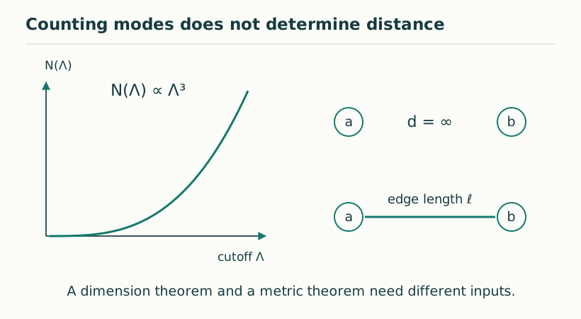
Figure 2. Counting modes does not determine distance. Spectral growth concerns how many modes lie below a cutoff. Distance concerns how observables vary under a normalized operator. The draft gives explicit examples in which the former is finite-dimensional while diagonal-state distances are infinite. View full size ↗
05What the construction explains for DTT
The graph block gives a rigorous interface between retained relational links and a metric on record states. It is an attractive target for a generative source because local comparison rules suffice to reconstruct global distances. However the graph, its edge lengths and persistence are currently supplied. A source law must explain why these links are selected, how they remain local under evolution and how their lengths relate to clocks. Exact recovery of a programmed graph metric should therefore be presented as a strong conditional result, followed by the separate formation and calibration questions.
06Disconnected components expose another assumption
Connectedness is essential for a finite distance between every vertex pair. If the graph has disconnected components, one can choose a function constant on each component but with arbitrarily different constants between components. Its commutator seminorm remains zero, so their distance is infinite. This is the graph analogue of missing comparison information. A single-source interpretation may motivate accessibility of all retained records, but that accessibility must appear in the operation graph or archive law. The metric theorem then quantifies the result: positive finite edge lengths and connected comparisons produce finite path distances, while inaccessible components remain metrically separated.
07Three diagnostics with different jobs
Spectral counting measures how the number of modes grows with frequency. A commutator seminorm measures which observables can vary between states while remaining Lipschitz bounded. An operational calibration connects these mathematical states and scales to actual records, distances and clocks. None of the three substitutes for the others. A compact auxiliary operator can have a clear counting exponent and nevertheless give infinite distances between selected localized states. Likewise a finite graph can have an exact distance without proving a smooth manifold limit or Lorentzian dynamics. Keeping these tests separate makes the reconstruction more informative and prevents a numerical plateau from being mistaken for complete spatial emergence.
Operator normalization is physical data once a spectral construction is used for measurement. Replacing D by aD multiplies its eigenvalues by a but divides its Connes distances by |a|. The counting exponent can remain unchanged while all calibrated lengths change. Likewise a bounded finite multiplicity changes a leading counting coefficient without changing its exponent. A proposed temporal explanation of geometry should therefore state both dimensionless structural results and dimensional calibrations. Agreement of an exponent with three is useful, but it cannot fix a ruler, a clock or their conversion by itself.
KEEP THE CONNECTION
Key ideas
The direct-sum edge normalization makes the distance theorem exact.
Shortest-path upper and lower bounds coincide.
Edge selection and physical length calibration remain separate inputs.
Scope of the argument. Exact finite weighted-graph metric result; not an automatic theorem for every hopping operator or a derivation of the graph itself.
Sources & further reading
dual_temporal_spectral_triples_v3.pdf — working draftpp. 15–16, Theorem 8.2
Source editions and catalogue entries
Working manuscript
Complex-Time Spectral Triples and the Separation of Spectral Dimension from Metric Distance
Draft file: dual_temporal_spectral_triples_v3.pdf
Working manuscript. Article-level references identify the consulted sections and the scope of the interpretation. No public URL was supplied for this exact manuscript version.