Explain the reduction of a finite linear model to states that can both be prepared and observed. Connect the quotient to the behavior actually accessible through a declared interface.
01The state an experiment can actually distinguish
A model may contain more variables than an experiment can prepare or observe. The operational holonomy draft asks which part of a finite linear model is fixed by its declared laboratory behavior. This is directly relevant to SMM/DTT: inner histories may carry distinctions that disappear in the outer record. The physically accessible state should therefore be derived from the available preparations, controls and future readouts. Removing inaccessible variables is not a denial of the source interpretation. It identifies which aspects of that interpretation can be supported by the specified interface.
02Controls and preparations play different roles
Consider a finite system with dx/dt=Ax+Bu and output y=Cx+Du. Independent preparation of an initial state is represented by a separate map E. Combining B and E into F=[B E] ensures that an accessible initial mode is not discarded merely because the ongoing control cannot excite it. The augmented transfer description includes both control response and preparation decay. This matters in atomic or clock models: preparing an excited phase state can expose a degree of freedom that ordinary continuous driving does not reach.
F=[B E]; Mₖ=CAᵏF.
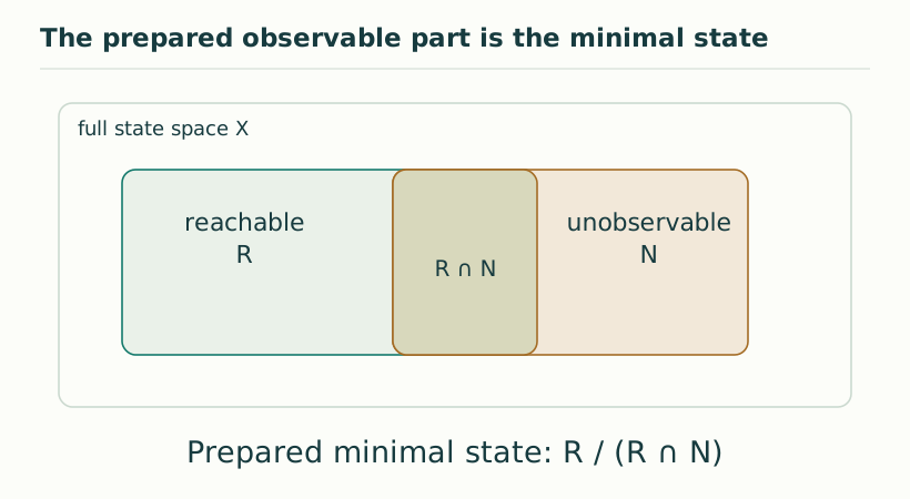
Figure 1. The prepared observable part is the minimal state. For a prepared linear interface, only reachable information that survives observational equivalence contributes to minimal behavior. The canonical state is R/(R∩N), not the entire hidden carrier. View full size ↗
03The reachable and unobservable spaces
The reachable space R is spanned by all AᵏFv. It contains states generated by the admitted control and preparation directions and subsequent evolution. The unobservable space N is the intersection of the kernels of CAᵏ: states whose entire future output vanishes. Both spaces are invariant under A. A state in R∩N can be prepared but cannot affect any admitted future reading. Such distinctions can be quotiented out without changing the declared behavior. States outside R cannot be prepared through the interface and need not appear in its minimal description.
R = span{Aᵏ im F : k≥0}; N = ⋂k≥0 ker(CAᵏ).
Xcan = R/(R∩N).
04Why this quotient is canonical
Restricting to R preserves every prepared response. Quotienting its unobservable part preserves every Markov parameter CAᵏF. The resulting realization is both reachable and observable. In finite linear realization theory, its dimension equals the rank of the block Hankel matrix made from those parameters, or equivalently the McMillan degree of the augmented transfer matrix. Any other minimal realization of the same interface differs only by an interface-preserving state similarity. The canonical object is therefore not one preferred coordinate array but the minimal behavior represented up to this exact equivalence.
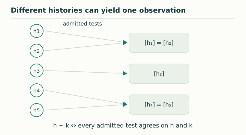
Figure 2. Different histories can yield one observation. The observational equivalence h ∼ k means that all admitted tests give the same result. Changing the test language can split an equivalence class and expose previously hidden distinctions. View full size ↗
05A two-mode worked example
Let A=diag(−1,−2), let the control excite the first coordinate, let independent preparation excite the second, and read their sum. The control-only response has one pole at −1. Once preparation is included, the observed behavior also contains a decay with pole −2, so its minimal dimension is two. Ignoring preparation would incorrectly declare the second mode unphysical. This example shows why any no-go argument for a proposed dual-time effect must state the full interface. A mode hidden from one control channel may be visible to a different allowed initialization.
B=e₁; E=e₂; C=(1,1).
Gaug(s)=((s+1)⁻¹, (s+2)⁻¹).
06The exact calculation is finite
Although R and N are written using all nonnegative powers of A, a finite n-dimensional realization needs only powers through n−1 to construct them. The Cayley–Hamilton identity expresses higher powers as combinations of those lower powers. Thus reachability and observability can be evaluated by finite block matrices once the exact system matrices are specified. This makes the quotient constructive rather than merely existential. With measured noisy data, however, exact zero singular values are replaced by uncertain small values, and choosing the model order becomes statistical inference. A source model can provide exact symbolic structure that helps this decision, but experimental precision alone does not certify an exact algebraic rank.
07What this teaches the source program
SMM/DTT can interpret X as a source-supported carrier and Xcan as the retained predictive record state. The quotient gives a rigorous meaning to “only completed observations are public” in this finite linear setting. It does not derive the chosen preparations or readout from the Monad, and it does not prove that all quantum or gravitational models admit the same reduction. A future source construction should specify the admitted interface and show which hidden distinctions remain predictively relevant. If a proposed temporal variable survives only outside Xcan, the present experiment cannot establish its independent empirical role.
KEEP THE CONNECTION
Key ideas
Independent preparations belong in the operational interface.
The minimal state is reachable behavior modulo unobservable distinctions.
Hidden generative variables need an accessible witness to carry empirical claims.
Scope of the argument. An exact result for finite-dimensional linear time-invariant prepared systems; it does not classify all nonlinear or quantum source models.
Sources & further reading
Operational Reduction and Exact Holonomy Localization for Finite Linear Dual-Time ModelsOperational_No_Go_Exact_Holonomy_Localization_v4.pdf, complete manuscript, pp.1–9
Source editions and catalogue entries
Working manuscript
Operational Reduction and Exact Holonomy Localization for Finite Linear Dual-Time Models
Working manuscript. Article-level references identify the consulted sections and the scope of the interpretation. No public URL was supplied for this exact manuscript version.