Turn the skeleton draft’s research direction into a practical analysis plan. Require more independent observables than fitted parameters and predeclare the cross-state prediction rules.
An atomic test is overconstrained when the model makes more independent predictions than it has freely fitted quantities. The word “independent” is essential: duplicated lines, exact transition-cycle identities and nearly proportional sensitivities do not create new information. Paper 14 proposes a design matrix for cross-state residuals. This provides a practical way to test SMM/DTT’s central aspiration that many observed quantities arise from one source law. The test should have enough freedom to represent its declared mechanism and little enough freedom that the pattern can genuinely fail.
02Build the parameter–observable map
Choose the effective operator family and compute its level matrix elements. Form a row for each reserved transition and a column for each unknown coefficient. Add nuisance columns for independently constrained conventional quantities such as nuclear parameters or calibration offsets. Label which coefficients are derived, externally measured or fitted within the test. The resulting matrix exposes accidental degeneracies: two physical explanations can be indistinguishable if they produce the same columns over the chosen channels. Improving precision alone cannot separate exactly identical directions.
r = Sc + Nη + ε, with covariance Σ.
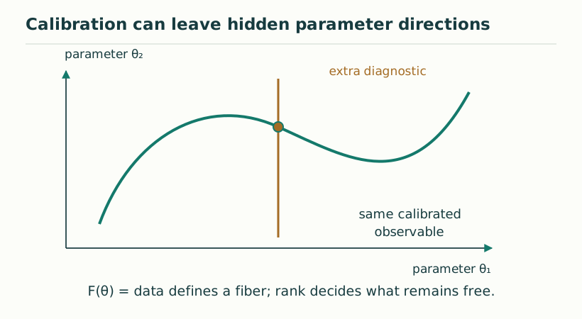
Figure 1. Calibration can leave hidden parameter directions. A fixed measurement may select a curve of models rather than one point. A genuine prediction must be constant on that calibration fiber, or require additional independently measured diagnostics. View full size ↗
03A small worked design
Imagine four independent residual channels and one proposed source amplitude. If the baseline is fully fixed, the vector r must lie near a one-dimensional line in four-dimensional data space. Three orthogonal combinations test the model without changing its amplitude. If two additional unconstrained nuisance directions are admitted, only one independent orthogonal combination remains. If the source column lies entirely in the nuisance span, the data cannot identify the source amplitude at all. This elementary geometry shows why a count of four lines and one named DTT parameter may overstate the actual test power.
04Use covariance-weighted residuals
With Gaussian errors and a justified covariance matrix, weighted least squares compares the residual vector to the model subspace using (r−Sc−Nη)ᵀΣ⁻¹(r−Sc−Nη), with suitable treatment of nuisance constraints. Exact singular directions should be removed or handled explicitly rather than inverted numerically without diagnosis. The nominal number of residual degrees of freedom is the data rank minus the rank of the fitted design, not necessarily the raw line count minus the number of parameter names. Strong nonlinearities or uncertain theory-error distributions may require a more careful inference procedure.
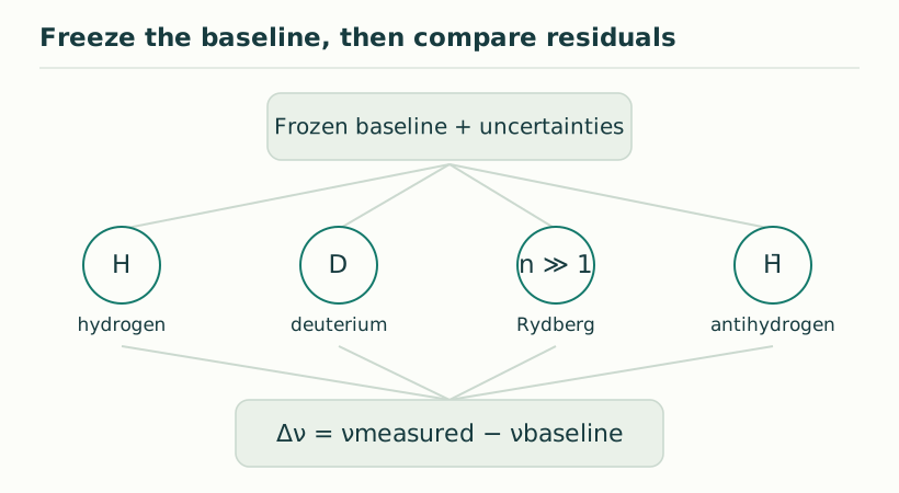
Figure 2. Freeze the baseline, then compare residuals. A differential test compares independently predicted and measured transitions across several systems. Shared nuisance effects can cancel only under a specified covariance model. The plotted markers are a design schematic, not data or DTT predictions. View full size ↗
05Predeclare what would reject the model
State the reserved channels, coefficient bounds, covariance treatment and test statistic before inspecting the final comparison. A failure can mean the operator family is wrong, the upstream normalization is wrong or the baseline is incomplete; the analysis should investigate those possibilities without silently changing the original prediction. If a revised model is introduced, preserve the earlier result and identify new tests. This practice is particularly important for structural-number programs because an apparently successful coefficient can conceal a choice among many grammars, branch conventions or normalization rules made after seeing data.
06A singular-value diagnostic for the design
After weighting by the inverse square root of the covariance, inspect the singular values of the fitted sensitivity matrix. A zero singular value means an exact combination of coefficients is unidentifiable; a very small one means noise strongly amplifies its uncertainty. For example, two shape columns proportional across every chosen transition cannot be separated regardless of how many times those transitions are measured. Adding a channel where the columns have a different ratio can restore rank. This gives a practical way to select complementary measurements before data collection. It also tests whether a proposed source relation genuinely reduces ambiguity or merely renames two existing correlated parameters.
07The link to the six-stage source program
An overconstrained test is most valuable when the source architecture predicts relations among operator coefficients. For example, a single completion law might fix the ratio of a contact-like term and a spin-sensitive term. That ratio should enter the matrix as a derived restriction, leaving fewer free directions. The six nested stages and outer completion must then be explicit enough that another reader can reproduce the restriction. The experimental design becomes an audit of the claimed common origin: do several physically different atomic channels obey the same source-imposed relation? The skeleton outlines this goal; the operator derivation and data analysis remain to be completed.
KEEP THE CONNECTION
Key ideas
Count independent model and nuisance directions, not just lines.
A design matrix makes shared source constraints testable.
Freeze the rejection criterion and preserve failed predictions.
Scope of the argument. A concrete analysis design for future work, with no fitted coefficients, significance level or successful result invented.
Sources & further reading
Hydrogen as a Differential Test of the Holonomy Fraction, skeleton outlinepaper14_hydrogen_differential_holonomy_tests.pdf, §§2–7, pp.3–9
Minimal hydrogen note: state and transition consistencysmm_dtt_minimal_hydrogen.pdf, §8.1, pp.6–7
Source editions and catalogue entries
Skeleton draft
Hydrogen as a Differential Test of the Holonomy Fraction
Working manuscript. Article-level references identify the consulted sections and the scope of the interpretation. No public URL was supplied for this exact manuscript version.