Introduce the finite-cell effective Hamiltonian and its explicit remainder. Explain why a controlled approximation needs a stated norm bound and an evolution-error estimate.
The gauge manuscript deliberately separates exact mathematics for a supplied singlet-binding Hamiltonian from a conditional SMM/DTT reconstruction of carriers, comparison rules and retained tensors. The static loop theorems use ordinary complex carrier spaces, positive penalties, hoppings and link matrices as inputs. The temporal interpretation asks whether one generative source and its completion records can select those inputs. Six nested inner stages are generative roles, not six separate clock axes or a pre-existing gauge multiplet. Exact solvability at the first layer is valuable, but it does not automatically close the selection problem at the second.
02An effective Hamiltonian needs an error statement
A formal virtual-loop expansion can suggest a magnetic interaction, but controlled dynamics requires a norm bound on the omitted operator and a stated preparation subspace. The draft constructs a finite-cell model with positive auxiliary penalties, small hopping ratio ε and bounded electric dispersion. The latter is capped through functional calculus while exact unitary link multiplication is retained. This is a precise regularization, whose volume and electric caps enter the sufficient smallness conditions.
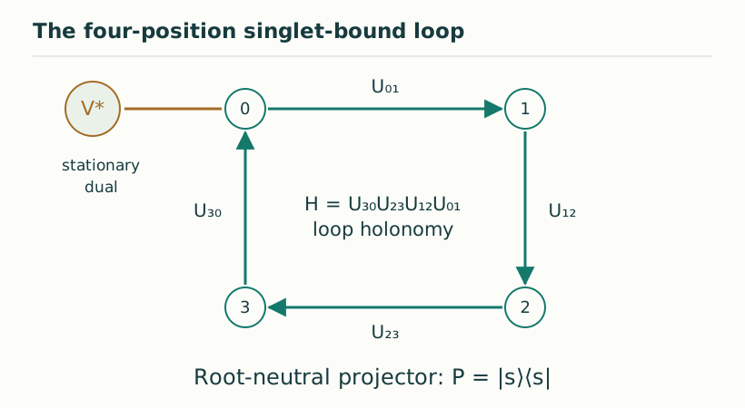
Figure 1. The four-position singlet-bound loop. A mobile carrier hops around four supplied positions while its stationary dual remains at the root. The root singlet penalty and the link holonomy determine the finite model response. This construction presupposes the lattice and carrier data. View full size ↗
03The leading loop term
For one static block at |t|/Δ<1/4, the expansion contains a second-order constant shift and a fourth-order holonomy term proportional to m−Re tr W. Its coefficient is 2t⁴/(mΔ³). Folded perturbative terms are needed: they cancel a holonomy-independent fourth-order contribution at W=I. Dropping them produces an incorrect target even before discussing errors. The full finite-volume construction includes electric effects at the stated order and bounds the remainder.
E_m(W)=−2t²/Δ+[2t⁴/(mΔ³)](m−Re tr W)+R_m
04Turn a norm error into a time interval
If ||H_eff−H_target||≤R, Duhamel’s formula bounds the difference of their unitary evolutions by |T|R/ℏ, capped by two. To guarantee error at most η, require |T|≤ηℏ/R. For example R=10⁻³ energy units with ℏ=1 gives a guaranteed error at most 0.1 through T=100 inverse-energy units. This is an illustrative bound, not a calculation for a particular gauge simulation. The manuscript emphasizes that conservative rigorous constants may give weak numerical guarantees even when computed errors are small.
Compressing links to a finite representation window generally destroys their exact unitarity. Boundary corrections can already appear at second order, before the desired magnetic term. The correct finite target therefore retains the compressed operator polynomials, or uses a padded window for specified coefficient matrix elements. Likewise the dynamical estimate applies to a dressed low-energy band; starting from bare singlets introduces a preparation error. For SMM/DTT these details distinguish an engineered completion mechanism with quantitative control from an analogy that merely resembles a gauge Hamiltonian.
06A rigorous bound can be valid and numerically uninformative
The manuscript explicitly notes parameter choices for which the conservative error estimate exceeds the maximum possible unitary difference and therefore reduces to the trivial bound two. This does not invalidate the asymptotic theorem, but it prevents using that bound as a practical accuracy certificate at those parameters. A simulation study should report both the proved envelope and directly computed errors, without substituting one for the other. For SMM/DTT the lesson is broader: a controlled approximation must specify where its control is quantitatively useful, especially before extrapolating a finite auxiliary construction to physical gauge dynamics.
07What a physical identification would require
A frame group, an invariant tensor and a loop response are mathematical structures. Identifying them with observed particle charges, interaction strengths and spacetime forces additionally requires matter statistics, chirality, dynamics, normalization and controlled scale matching. A connection can be flat even when its allowed structure group is large. A finite auxiliary gap can be positive without establishing a continuum Yang–Mills mass gap. The SMM/DTT programme becomes sharper when these distinctions are retained: a proposed temporal source law can then be asked to reproduce specific carriers and coefficients rather than receiving credit for empirical physics merely because familiar group labels appear.
Gauge-invariant density matrices and neutral amplitudes are different notions. Averaging a density matrix over frames can leave a maximally mixed state in a nontrivial charged representation. Averaging amplitudes coherently projects onto invariant vectors and can instead select a singlet sector. A completion mechanism must specify which operation it implements and where its reference carrier resides. This distinction matters when interpreting a static singlet calculation as a physically generated neutral sector: symmetry of the Hamiltonian preserves a chosen sector but does not automatically prepare it.
KEEP THE CONNECTION
Key ideas
A controlled approximation states both a remainder norm and an evolution-time bound.
Folded terms and representation-boundary effects cannot be omitted.
Finite-volume dressed-band control is not a continuum-uniform theorem.
Scope of the argument. Controlled finite-cell regularization; constants are not claimed uniform in volume, electric cutoff or continuum limit.
Sources & further reading
Gauge_Structure_Temporal_Completion_v20(2).pdf — working draftpp. 11–16, Theorems 2.5–2.6 and §2.3.1
Source editions and catalogue entries
Working manuscript
Gauge Structure from Temporal Completion in SMM/DTT — Version 20
Working manuscript. Article-level references identify the consulted sections and the scope of the interpretation. No public URL was supplied for this exact manuscript version.