
In this article
- Local and global questions are different
- Curvature gives the local boundaries
- The three thresholds have a strict order
- A worked finite-cycle comparison
- Why corrections need a safety margin
- The conceptual lesson for completion
Explain why local stability boundaries and global phase selection answer different questions. Use the finite-cycle model to organize the possible competing extrema.
A stationary point can resist small perturbations while another configuration has lower energy. Local stability asks about the nearby shape of the potential; global selection compares the entire allowed configuration space. The finite-cycle SU(2) model offers a clean example. The center becomes locally stable before it becomes the global minimum, and the endpoint configurations can remain locally stable after the center wins globally. This metastability is not a defect in the calculation. It is a physical distinction that any proposed completion rule must respect when it claims to select a stable holonomy.
For UM,h, the second derivative at the center is 2[h−hloc(M)], while at the endpoints it is 2[hend(M)−h]. Positive curvature supplies local stability, with endpoints treated relative to the Weyl chamber. The draft gives closed expressions in β=π/(2M). At a boundary where curvature vanishes, higher-order terms must be inspected; zero curvature alone does not establish a local minimum. The complete classification in the manuscript handles those marginal cases using the same concavity structure that proves the global result.
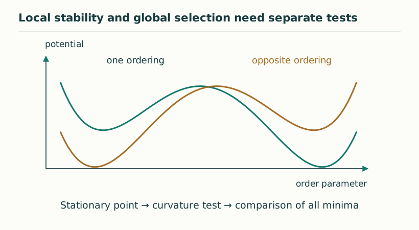
The draft proves 0<hloc<hc<hend. Between hloc and hc, the center is locally stable but the endpoints are globally preferred. Between hc and hend, the center is globally preferred while the endpoints remain metastable. At hc they coexist with equal global energy. This makes it clear why reporting only a positive central curvature would overstate selection. A source model that produces h slightly above hloc has created a local well, not necessarily the preferred completed configuration.
At M=8, the three thresholds are approximately 0.174451, 0.213836 and 0.342197. Choosing h=0.19 makes the center locally stable but leaves the endpoints globally preferred. Choosing h=0.25 selects the center globally while retaining local endpoint minima. Choosing h=0.36 removes that endpoint local stability. These examples use one fixed leading effective potential. They should not be read as predictions of transition rates: escape from a metastable well requires dynamics, fluctuations and an energy or action barrier analysis beyond the location of minima.
The continuum limits are 1/6, π²/48 and 1/3 respectively. Higher perturbative and nonperturbative terms can shift the effective potential and its boundaries. A proposed source mechanism should therefore produce a controlled margin above the global threshold, not simply hit the one-loop coexistence point. The draft supplies a sufficient robustness condition for a symmetric twice-differentiable remainder in terms of its second-derivative norm. Such a condition becomes useful only when the microscopic remainder is actually bounded. An uncomputed correction cannot be assumed small because the leading picture is appealing.
SMM/DTT often invokes stable completion as the emergence of a persistent outer record. The finite potential shows that “stable” must be defined: locally resistant, globally preferred, dynamically reachable and long-lived are different properties. A completion filter could select a metastable state by protocol even when it is not the equilibrium minimum. An autonomous source law must explain its selection and resource or time scale. The six nested stages may provide a structured path through configurations, but the potential does not derive that path. This article therefore links the mathematical phase diagram to a sharper vocabulary for physical record formation.
KEEP THE CONNECTION
Scope of the argument. Local and global results apply to the declared leading potential; transition rates and full dynamical selection are not derived.
Draft file: yang_mills_holonomy_monopoles_v7(1).pdf
Working manuscript. Article-level references identify the consulted sections and the scope of the interpretation. No public URL was supplied for this exact manuscript version.
Source register →