
In this article
- Partial progress contains measurable information
- The binomial stage law
- The complete observation alphabet
- Derive the Fisher information
- Calibration and recurrence matter
- A finite example
- The connection to inner and outer time
Use the autonomous-history construction to connect partial progress with prefix probabilities and clock Fisher information. Explain what can be learned before a final record is complete.
A final completed record is not the only observable of an autonomous generator. The history clock can reveal how far the program has progressed, and that distribution can be used to estimate the evolution parameter within a calibrated branch. The draft computes both prefix probabilities and clock Fisher information exactly.
For SMM/DTT this clarifies two temporal roles without introducing two independent axes. Inner progress is a state of the generating device; outer access is a specified measurement of its stage, flag, or completed file. Different measurements retain different information.
In the engineered history clock, J takes values 0 through L with binomial parameter p_s=sin²(ωs/2). The mean stage is Lp_s and its variance is Lp_s(1−p_s). The distribution moves from stage zero to stage L on 0≤s≤π/ω.
A prefix completed at stage k is certified with probability S_k(s)=Pr(J≥k). This is a binomial upper tail. It is increasing on the prepared forward branch, but it is not the probability distribution of an unmeasured classical first-passage time. The underlying state generally remains coherent across stages.
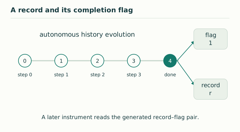
With two prefix flags at thresholds k₁<k₂, the possible record sectors are absent, first only, and both. Their probabilities are 1−S_k₁, S_k₁−S_k₂, and S_k₂. These add to one and keep incomplete outcomes visible.
Conditioning only on the final complete sector can conceal a substantial unfinished fraction. A useful experiment should compare the entire sector distribution before analyzing successful-file contents. In the ideal construction, the sector probabilities depend on the clock dynamics while the completed data probabilities depend on the encoded work.
For a binomial distribution with parameter p, the Fisher information in p is L/[p(1−p)]. Here dp_s/ds=(ω/2)sin(ωs), and p_s(1−p_s)=sin²(ωs)/4. Applying the chain rule gives I_s=Lω² for interior points of the forward branch.
For ν independent prepared runs, a locally unbiased estimator therefore satisfies Var(ŝ)≥1/(νLω²). The formula has a clear resource interpretation: more clock capacity and more repetitions improve local precision. It is not a derivation of an absolute action scale or a universal quantum limit for all clocks.
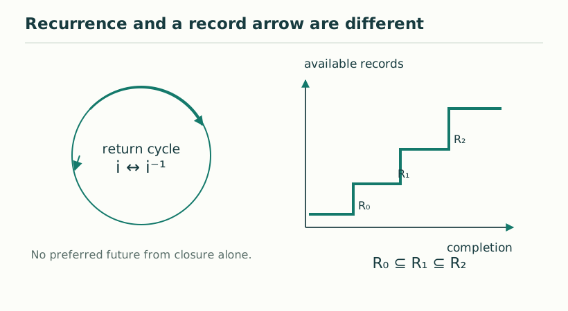
A natural reading assigned to stage j is T(j)=(2/ω)arcsin√(j/L). It inverts the mean-parameter relation on the declared forward branch. The frequency ω must be independently calibrated, and the reading is noisy; a single stage outcome does not equal s exactly.
Outside the branch, recurrence creates ambiguity because the same p_s occurs at multiple parameter values. The local Fisher-information result does not remove that global ambiguity. The endpoint statistical parametrization also needs care, so the quoted local bound is stated for interior times.
For L=16, the local Fisher information is 16ω². With ν independent runs, the standard-deviation lower bound is 1/(4ω√ν). A prefix at k=8 is approximately halfway through its transition near p_s=1/2, while the final-stage probability is then only (1/2)^16.
Thus a clock can give substantial information about progress while the full program is unlikely to have completed. Progress estimation, completion certification, and final data accuracy are distinct tasks. Their resources should not be collapsed into one number called the tick count.
The record-oriented interpretation treats an observed completed prefix as evidence that the required ordered composition has been realized. It does not assert that stage labels are independent physical times. The six nested functional levels can organize the program but are different from its gate count K and clock length L.
A complete final file may even discard the stage information that made the clock informative. The distinction between a readable record and a predictive or temporal state is therefore visible within the same model. SMM/DTT can use this calculation as an operational benchmark while keeping calibration, recurrence, and resource limitations explicit.
KEEP THE CONNECTION
Scope of the argument. Exact engineered-clock statistics; the precision bound is local, calibrated, and model dependent.
Draft file: SMM_DTT_Autonomous_Records_Free_Field_Limits_v10(6).pdf
Working manuscript. Article-level references identify the consulted sections and the scope of the interpretation. No public URL was supplied for this exact manuscript version.
Source register →