Physical quantum clocks: finite resources and temporal completion
A physical clock is a quantum system with finite energy, distinguishable states and a readable record. DTT’s inner/outer distinction becomes stronger when these resources are part of the source model. This guide connects completion to conditional events, works through a clock-precision bound, and identifies the missing mechanism behind a universal geometry–clock relation.
A time parameter in an equation can be arbitrarily precise, but a physical clock has a state, a Hamiltonian and a measurement. Its reading is inferred from a change that can be distinguished from noise and from other possible times. Quantum-clock research studies those constraints directly, including situations where clocks interact with gravitating systems and the localization of an event depends on the chosen reference.
DTT proposes that outer time orders accessible completions of inner generation. This is potentially a physical-clock statement, but only if the completion counter is implemented by a material degree of freedom with a specified interaction and resource budget. Six nested inner levels describe the architecture producing the record; they are not six ideal clock parameters. The source should explain how a readable clock emerges and why it remains compatible with the matter it times. [1][2]
02Worked example: a two-level clock
Take H=(ħω/2)σz and prepare the equal superposition of its two energy eigenstates. The relative phase evolves as ωt, so a suitable measurement can estimate t locally. The energy standard deviation is ΔH=ħω/2. For a pure state under unitary evolution, the quantum Fisher information for t is FQ=4(ΔH)²/ħ²=ω².
For N independent preparations and an appropriate locally unbiased estimator, the quantum Cramér–Rao bound gives δt≥1/(ω√N). If ω=2π×10⁹ s⁻¹ and N=10⁶, the bound is approximately 1.59×10⁻¹³ s. This is an ideal local estimation limit, not a guarantee that any real clock achieves that precision. Measurement choice, noise, prior ambiguity and interaction with the timed system still matter.
FQ=4(ΔH)²/ħ²=ω²; δt≥1/(ω√N) for N independent ideal trials.
The bound assumes a pure unitary clock state and local unbiased estimation. It is not a universal single-shot timing bound for arbitrary clocks.
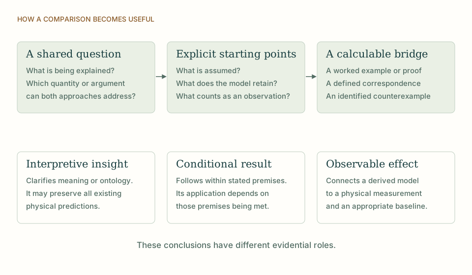
A comparison that reaches a definite conclusion. Begin with the same question, identify what each approach assumes, and compare a shared result. An interpretation, a conditional theorem and an observable deviation have different evidential roles. View full size ↗
03Precision is not unambiguous duration
The same two-level clock repeats its phase every 2π/ω. An arbitrarily accurate phase estimate does not identify which cycle has elapsed. A long-duration clock therefore needs retained memory, additional frequencies or an external prior. This is a direct point of contact with DTT completion: an outer record must retain enough information to distinguish completed events, not merely produce a rapidly rotating phase.
The memory has a physical role. It can preserve the count of completed cycles and certify which event triggered the record. If the source overwrites that memory at each inner step, its phase may be precise while its accessible history is ambiguous. Conversely, a stable counter can order events with coarse timing resolution. These are different clock resources and should be represented separately in an autonomous model.
04The source origin of universal clock response
SMM/DTT can frame this universality as a common origin of clock production and motion. The same nested generative process would determine both a completed material transition and the geometry against which that transition is compared. The seventh, outer role is the readable clock record; the six inner levels are not six separately observable clocks.
The constructive issue is protection. If the model simply assigns each species a frequency ωₛ and rescales it by a chosen function of potential, universal redshift has been assumed. A stronger model derives a common multiplicative response from a symmetry or a shared conserved source quantity, while allowing different transition energies. That would explain how clocks differ in their natural periods yet agree on elapsed proper time after calibration.
05Why the dimension–clock relation needs a mechanism
A record-refinement model can yield a geometric exponent D=lnB/ln(1/r), while a material oscillator has a frequency set by its Hamiltonian. Those quantities can vary independently. Defining the oscillator's reading to equal D does not derive a relation between geometry and clocks.
A stronger DTT construction would couple both observables to the same source trajectory. For example, a conserved source charge might determine the work needed to create a branch and the phase accumulated by a physical transducer. The model would then have to show why changing B and r changes the clock response without retuning the oscillator by hand. The protection of that relation under perturbations is part of the result.
The quantum-clock calculation makes the resource question explicit. A faster or more precise transducer requires an appropriate energy spread, repeated preparation or memory. A source theory cannot obtain an arbitrarily accurate universal clock solely by increasing an unobserved iteration rate. Its physical budget must accompany the claimed geometry–clock equality.
06Events and conditional probabilities
A clock-defined event can be modeled as an operation applied when the clock lies in a specified reading range. Its probability is then a joint or conditional probability involving the clock and the system. If the clock becomes entangled with matter or geometry, the effective event timing can broaden or become reference dependent. The cited quantum-clock framework studies such relations without requiring a second ordinary time axis.
DTT can add a generative account of the event and its completion flag. The flag should be produced by the same autonomous interaction, and all outcomes must retain normalized probabilities. A successful completion selected by postselection must include its probability and resource cost. This is the difference between a physical event instrument and an abstract instruction to read the clock at the desired moment. [1]
07The most useful research conclusion
A strong temporal-source clock model would combine a finite Hamiltonian, retained cycle memory, a completion instrument and an independently defined geometric observable. It would calculate their joint statistics and identify a protected relation. This could establish a real piece of DTT even before a full theory of spacetime exists. The useful comparison with quantum clocks is that it replaces an ideal hidden time parameter with a physical device whose precision, ambiguity and interactions can all be analyzed.
THE SAME QUESTION, DIFFERENT STARTING POINTS
The comparison at a glance
Question
SMM/DTT
Quantum-clock precision and event localization
Clock variable
Outer time should be a readable completion record generated by the source.
A quantum clock has a state, Hamiltonian and measurement.
Resources
Energy spread, memory and success probability belong to the source budget.
Precision and duration are limited by distinguishability and retained information.
Novel relation
Geometry and clock readings should be jointly constrained without retuning.
Conditional timing alone does not determine a geometric scaling exponent.
KEEP THE CONNECTION
Key ideas
Outer time should be a readable completion record generated by the source.
Energy spread, memory and success probability belong to the source budget.
Geometry and clock readings should be jointly constrained without retuning.
Develops the source construction or operational distinction used in this comparison.
Sources and further reading
References support the comparator and the specific mathematical or interpretive claims indicated. SMM/DTT connections are developed in the analysis above.