Singularity resolution and geodesic completeness: SMM/DTT and Causal set theory
Does discrete re-creation remove physical singularities, or merely replace divergent variables by a bounded description? This article compares the source-based construction with Causal set theory, identifies their strongest point of contact, and works through a concrete example that separates a valid mathematical result from the further physical relation needed to explain observations.
A spacetime singularity is not simply a place where a selected density becomes large. In general relativity, geodesic incompleteness means that a freely falling trajectory can end after a finite proper time without extension inside the spacetime. Curvature may diverge, but finite curvature alone does not guarantee that all physical trajectories continue uniquely.
A quantum model can address this problem in several ways: a bounce may replace a classical collapse, a wave function may remain regular, or geometry may cease to be an appropriate description. Each possibility requires a criterion for continuing physical observables. The word resolution is therefore meaningful only when the model states what replaces the classical trajectory and whether its evolution remains well defined. [1][2]
02The SMM/DTT contribution
DTT offers the idea that apparent spatial breakdown could reflect a change in the completion of inner generative processes. If no completed record corresponds to a classical singular geometry, the classical divergence may be outside the domain of the readout. That is a potentially coherent interpretation, but exclusion from the output catalogue is not yet a dynamical account of what an infalling system experiences.
The six nested inner levels may continue to operate even when the outer geometric description fails. To turn that suggestion into physics, the model needs a well-defined state across the transition, conserved probabilities or a specified open-system evolution, and a rule connecting records before and after it. The Single Monad's ontological continuity cannot substitute for mathematical existence and uniqueness.
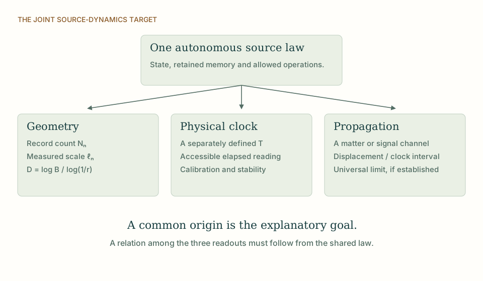
Geometry, clocks and propagation as independent readouts. A single source model should explain the relation between separately defined measurements. Sharing a diagram does not impose that relation. View full size ↗
03How Causal set theory frames the problem
Causal set theory replaces continuum spacetime by a locally finite partial order. Order represents causal precedence and counting supplies a volume measure in an appropriate continuum approximation. A stochastic embedding can preserve Lorentz symmetry statistically without introducing a fixed regular grid. The difficult dynamical question is why the resulting order should approximate a suitable manifold.
This is close to DTT in giving event structure explanatory priority over an assumed spatial stage. The important difference is that a partial order is already an explicit relational object, whereas a source ontology must explain how records and their order are generated. A total sequence of source operations and the partial order accessible to observers are not automatically identical. [3]
04Where the mechanisms agree and differ
Causal set discreteness removes the assumption that every physical region contains a continuum of points, but it does not automatically remove all singular behavior. A generated order can end, fail to approximate a manifold, or give pathological propagation. DTT has a closely related issue: a source can keep producing records while those records cease to support an acceptable observer history.
The comparison is therefore about criteria for extension. In an order-based model, one can ask whether causal paths and matter amplitudes continue consistently. In DTT, one must additionally specify which inner histories yield the accessible continuation and whether completion loses information. Six nested levels do not ensure uniqueness or stability. The bounce example below is a continuum effective illustration, so it cannot be assumed to describe every discrete causal construction. Its value is to expose the kind of dynamical sign change needed to replace collapse with expansion. A strong temporal model would derive an analogous continuation criterion directly from source dynamics, then show when a smooth metric emerges on both sides. This would turn source persistence into a testable mathematical statement about physical evolution. [3]
05Worked example: assumptions, calculation and result
A common illustrative bounce equation is H²=(8πG/3)ρ(1−ρ/ρc), with ρ treated as mass density and ρc a positive critical density. It gives H=0 at ρ=ρc. For a fluid with w=p/(ρc²), energy conservation gives ρ̇=−3Hρ(1+w). Away from H=0, differentiating and continuing smoothly yields Ḣ=−4πGρ(1+w)(1−2ρ/ρc).
At ρ=ρc and w>−1, Ḣ=4πGρc(1+w)>0: contraction turns to expansion. The algebra identifies a bounce within this effective homogeneous model. It does not derive the equation from DTT, establish inhomogeneous stability, or prove geodesic completeness in the full theory. Those distinctions prevent a useful worked mechanism from becoming an overstated universal conclusion. [1][2]
H²=(8πG/3)ρ(1−ρ/ρc); at ρ=ρc, H=0 and Ḣ=4πGρc(1+w)>0 for w>−1.
ρ and ρc are mass densities, H has units s⁻¹, and w is dimensionless. This is an illustrative effective bounce law.
06An independent operational check
A bounce of the average scale factor need not bound fluctuations or tidal observables. Two states can share the same mean volume while one has a broad distribution extending into a problematic regime. A physical resolution therefore concerns the state and its observables, not just a plotted mean trajectory. The source-to-record map can make this precise by identifying what an internal clock and a matter probe would read across the transition. A well-defined continuation may exist even when no smooth metric does, but the model must state its replacement measurements rather than relying on the continued existence of an unobserved source alone.
07What follows from the comparison
A strong source-based result would specify which observables remain finite and how their evolution passes through a region where classical geometry fails. A bounded operator spectrum can help, but its dynamics and physical interpretation still matter. Comparison with published bounce models is most useful when it exposes these separate tasks and identifies a smaller theorem that can actually be proved.
THE SAME QUESTION, DIFFERENT STARTING POINTS
The comparison at a glance
Question
SMM/DTT
Causal set theory
Starting physical structure
One nonspatial source; six nested inner functional levels produce records accessible through outer completion.
Locally finite causal order with element counting as an approximate volume measure.
The central mechanism in this topic
A continuing source must yield consistent causal and material records across the transition.
Discrete causal structure needs its own criterion for extension and propagation regularity.
How the claim is made operational
A source-to-record map must define geometry, material response and physical clocks with shared inputs.
Order invariants, stochastic dynamics and continuum-approximation criteria.
Meaning of agreement
Agreement is a compatibility result; a source-selected relation or fixed residual would add explanatory content.
The stated framework provides a benchmark within its own assumptions and established domain.
KEEP THE CONNECTION
Key ideas
Discreteness removes some continuum assumptions but does not by itself prove physical completeness.
The worked example establishes only the result stated under its explicit assumptions.
Six nested inner levels describe one generative organization; outer time orders accessible completion.
Develops the source construction or operational distinction used in this comparison.
Sources and further reading
References support the comparator and the specific mathematical or interpretive claims indicated. SMM/DTT connections are developed in the analysis above.