SMM/DTT as an effective theory: matching a source to observables
A source theory becomes comparable with established physics through an explicit map to low-energy observables. Effective field theory supplies that map without assuming that every microscopic detail is directly measurable. This article explains how DTT can use matching to preserve its distinctive generative claims while making concrete predictions and identifying which freedoms remain.
An effective theory lists the fields or observables relevant in a stated regime and the interactions allowed by its symmetries. Higher-order terms encode short-distance physics through coefficients. The theory can be predictive at low energy even when the ultimate microscopic description is unknown. Donoghue's treatment of gravity is a useful example: low-energy quantum effects can be separated from unknown ultraviolet contributions.
DTT aims to supply a microscopic source for those effective fields, clocks and geometry. The six nested inner levels describe the production architecture, while outer completion defines the accessible sector. Matching asks which effective action or response reproduces the source's observable amplitudes in a controlled regime. It is not a surrender of the source ontology; it is the step that makes that ontology physically assessable. [1]
02A simple matching calculation
Suppose a low-momentum source calculation yields a scalar inverse propagator Γ(p)=Zp²+m0²+a p⁴/M²+… in Euclidean notation. Canonical normalization φcan=√Z φ gives a physical quadratic mass parameter m²=m0²/Z and a higher-derivative coefficient a/Z. The raw coefficient m0 is therefore not yet the measured mass parameter.
If the source also couples φ to another field, that interaction rescales as well. Matching must treat all terms consistently. A model that reads a mass from one unnormalized operator and a coupling from another can manufacture a relation that disappears after canonical normalization. The source's positive task is to fix invariant combinations such as m0²/Z and the corresponding normalized interactions.
Γ(p)=Zp²+m0²+a p⁴/M²+…; φcan=√Zφ ⇒ m²=m0²/Z.
Natural units; p and M have energy units. Z>0 is assumed, and the expansion is used only for momenta small compared with M.
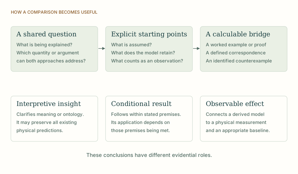
A comparison that reaches a definite conclusion. Begin with the same question, identify what each approach assumes, and compare a shared result. An interpretation, a conditional theorem and an observable deviation have different evidential roles. View full size ↗
03Matching the gravitational coefficient
Use natural units c=ħ=1 and consider S=∫d⁴x√−g[(M²/2)R−ρΛ+Lₘ]. With the usual definition Tₐᵦ=−2(δSₘ/δgᵃᵇ)/√−g and suitable boundary terms, variation gives M²Gₐᵦ+ρΛgₐᵦ=Tₐᵦ. Thus M²=1/(8πG) and Λ=ρΛ/M² reproduce the conventional Einstein equation.
The Bianchi identity ∇ᵃGₐᵦ=0 implies ∇ᵃTₐᵦ=0 when M and ρΛ are constant. If a proposed temporal rate makes M position dependent, derivatives of M enter the variation and the simple equation is no longer correct. This small calculation makes a useful diagnostic: a varying generative parameter cannot simply be inserted into a constant-coupling equation without accounting for its dynamics and energy exchange. [1][4][5]
M²Gₐᵦ+ρΛgₐᵦ=Tₐᵦ; M²=1/(8πG); Λ=ρΛ/M² (c=ħ=1).
M has mass dimension 1, R dimension 2, and ρΛ dimension 4. Appropriate boundary conditions and boundary terms are understood.
04What must be generated together
A source model may reproduce a free field while leaving interactions unconstrained. It may generate a graph while assuming a physical clock. It may derive a neutral projector while choosing its energy coefficient independently. These are valid partial constructions, but they should not be combined into a claim of one inevitable theory unless the same update links their free choices.
Effective matching makes those choices visible. It identifies which source parameter controls each observable coefficient and which relations remain after field redefinitions. Six nested inner levels can be a genuine organizing principle if they enforce such relations. A single controller running independently selected subrules does not reduce the effective parameter freedom.
The strongest target is therefore a small set of shared coefficients with several consequences. A source-selected transport operator might determine a clock response and a wave correction together. A completion rule might constrain a gauge kinetic coefficient and a neutral-sector observable. Each relation can be tested mathematically before any claim of complete unification is made.
05Separating known limits from new effects
The leading effective action should reproduce the established regime relevant to the calculation. A new correction is then the difference predicted by the source with parameters fixed in advance. It must have a defined operator, scale dependence and domain of validity. If the correction can be removed by a field redefinition or a common clock calibration, it is not an independent observable.
Conversely, a source theorem can be valuable even when it predicts no deviation. Explaining why all material species share a cone or why one phase normalization is universal would reduce assumptions in the effective theory. The advance lies in the derived restriction, not necessarily in a large anomaly. [1][2]
06Vacuum energy remains a separate coefficient
The vacuum term and the curvature term must be tracked separately. A model can produce a plausible coefficient of R while leaving a large additive vacuum energy. Normalized transition probabilities may be insensitive to that additive constant, but gravity couples to the effective stress-energy associated with it. Thus a successful response calculation for G does not automatically solve the cosmological constant problem. This separation is particularly useful for temporal spectral proposals: the same operator can contribute several effective coefficients, and each requires its own matching and stability argument. A common source is valuable when it constrains their relations, not when distinct coefficients are conflated. [3][1]
07A concrete role for the SMM/DTT programme
The source ontology proposes one origin for what effective theory normally treats as separate ingredients: geometry, matter, clocks and retained records. Matching provides a disciplined way to assess that proposal. A successful model would identify the state space and autonomous update, calculate a set of accessible responses, and show that their effective coefficients obey a nontrivial relation. The relation should remain meaningful under changes of representation and controlled refinement.
This is a realistic standard for a strong new paper or website claim. A limited but complete matching result can be more important than a broad list of familiar equations with independent assumptions. It gives readers a concrete mechanism, an observable consequence and a clear account of what has actually been derived.
THE SAME QUESTION, DIFFERENT STARTING POINTS
The comparison at a glance
Question
SMM/DTT
Effective field theory matching
Microscopic content
One source should generate geometry, matter and clock response jointly.
Effective fields and allowed operators describe a specified observable regime.
Matching
Source amplitudes determine normalized coefficients and relations.
Field redefinitions and canonical normalization identify physical combinations.
New physics
A fixed residual or protected relation must survive calibration.
The baseline and correction are separated within a controlled expansion.
KEEP THE CONNECTION
Key ideas
One source should generate geometry, matter and clock response jointly.
Source amplitudes determine normalized coefficients and relations.
A fixed residual or protected relation must survive calibration.
Develops the source construction or operational distinction used in this comparison.
Sources and further reading
References support the comparator and the specific mathematical or interpretive claims indicated. SMM/DTT connections are developed in the analysis above.