Temporal discreteness and Lorentz-violation bounds
A discrete inner process need not produce an observable preferred frame, and a hyperbolic notation does not guarantee Lorentz symmetry. This article explains how DTT should be compared with precision bounds: first derive the effective operator and its clock interpretation, then identify the measurement that constrains its coefficient.
Lorentz transformations preserve the interval between events and relate the readings of moving rods and clocks. In one spatial dimension they can be written using hyperbolic functions of a rapidity. That elegant mathematical form is necessary for the usual boost group, but its physical interpretation also needs a common signal cone and transformation laws for material measuring devices.
A split-complex number uses a unit j with j²=+1, whereas ordinary quantum phase uses i²=−1. The two algebras have different norms and different exponential maps. Neither notation, by itself, creates a second measured time or proves a Wick rotation is a physical event. A precise comparison keeps algebra, coordinate change and dynamical observer transformation separate. [2][1]
02The source-based interpretation
DTT's inner/outer distinction invites a hyperbolic description because generation and accessible completion are not interchangeable roles. A split-complex construction can encode an invariant quadratic relation between selected variables. Its value is that the invariant can be stated and checked explicitly, rather than inferred from a picture of perpendicular axes.
The decisive next identification is operational: the variables must be generated clock and distance observables, and the proposed transformations must act on actual histories and interactions. Six nested inner levels do not add six boost directions. If the same update supports a single outer causal cone and three spatial readout directions, the construction can be assessed against 3+1-dimensional Lorentz symmetry without reinterpreting functional nesting as a higher-dimensional spacetime.
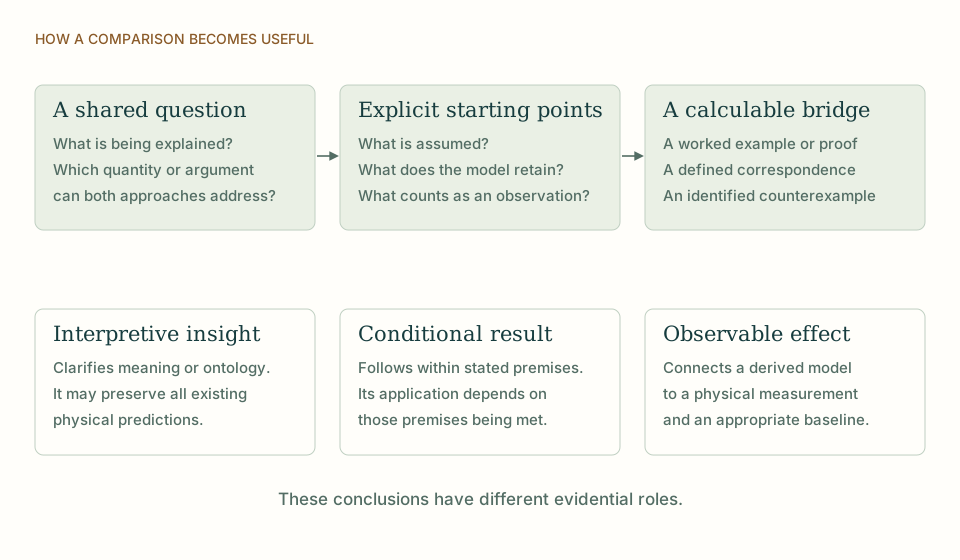
A comparison that reaches a definite conclusion. Begin with the same question, identify what each approach assumes, and compare a shared result. An interpretation, a conditional theorem and an observable deviation have different evidential roles. View full size ↗
03What a bound actually constrains
Published Lorentz and CPT tests constrain particular operators, species, polarization combinations and reference-frame components. There is no single number that limits every possible form of temporal discreteness. A photon dispersion coefficient, a spin-dependent fermion coupling and a difference between material clock sensitivities are different physical parameters.
DTT must therefore translate its source dynamics into an effective observable before applying a bound. A source update may leave an exact Lorentz-invariant outer sector, or it may introduce a preferred tensor or a modified dispersion law. Both are mathematically possible. Six nested inner levels do not decide which occurs. The source's transformation law and the way matter reads its output are the decisive ingredients. [1]
04Worked dispersive example
Consider the illustrative massless dispersion relation E²=p²c²[1+ξ(pc/M)²], with |ξ|(pc/M)²≪1 and M an energy scale. Expanding gives E≈pc[1+(ξ/2)(pc/M)²]. Differentiating with respect to p yields vg≈c[1+(3ξ/2)(pc/M)²]. The leading fractional group-speed correction therefore scales quadratically with energy in this toy model.
Two wave packets of different energies can accumulate a relative delay over a long path. Its interpretation requires the emission lag and propagation environment to be modeled. The coefficient ξ is not predicted here by DTT; the example shows how a source-derived correction would become a quantity to constrain. A different operator could give a different energy power or polarization dependence, so the bound cannot be transferred indiscriminately.
E²=p²c²[1+ξ(pc/M)²] ⇒ vg/c≈1+(3ξ/2)(pc/M)².
M has energy units; ξ is dimensionless. This is a perturbative illustrative operator, used only where the correction is small and the physical branch is stable.
05A nondispersive multimessenger benchmark
For a simple nondispersive propagation comparison, take a source distance of 40 megaparsecs and an arrival-time difference of 1.7 s. Since 1 Mpc≈3.086×10²² m, the travel time is approximately 4.12×10¹⁵ s. Dividing gives |Δv|/c≈4.1×10⁻¹⁶ if the entire delay is attributed to propagation.
This arithmetic is only an illustrative inference. Electromagnetic and gravitational signals can leave the source at different times, and cosmological propagation requires a more careful treatment. The published GW170817 analysis incorporates astrophysical assumptions in its bounds. A DTT wave-speed claim must specify those same assumptions and cannot equate the observed arrival delay directly with an intrinsic inner-time lag. [4][2][5]
Δv/c≈Δt/(D/c). For D=40 Mpc and Δt=1.7 s, the propagation-only estimate is 4.1×10⁻¹⁶.
D is the source distance in this approximation; the sign and magnitude of an intrinsic emission lag are separate inputs.
06Why hidden production order is not automatically observable
A total sequence of source operations may carry more ordering information than the outer causal record. If all observable probabilities are invariant under changes of that hidden ordering, it need not define a measurable preferred frame. If the ordering changes transition rates or signal propagation, it has physical consequences and must be confronted with the corresponding tests.
This distinction gives DTT a clear mathematical target. The source can be studied for an exact symmetry of its accessible sector, or for a controlled small breaking. In either case, the clock variable used to state the correction must be operational. A rescaling of an unobserved iteration counter is not a measured change in light speed. Likewise, a delay in a detector's completion process is not necessarily a vacuum propagation effect. [3][2]
07A stronger form of prediction
The most informative temporal signature would relate several coefficients through one source mechanism. For example, a specified update could link a wave-dispersion term to a clock response or a direction-dependent transport correction. Such a relation reduces the freedom to fit each experiment separately.
If the source instead protects exact Lorentz invariance, that can be a valuable explanatory result even when it predicts no violation. It shows why microscopic generation does not leak a preferred frame into outer measurements. The comparison with bounds then establishes compatibility rather than experimental confirmation of DTT. Both outcomes are scientifically meaningful when the assumptions and observable maps are explicit.
THE SAME QUESTION, DIFFERENT STARTING POINTS
The comparison at a glance
Question
SMM/DTT
Effective operators and Lorentz tests
Discreteness
A source update may preserve or break accessible Lorentz symmetry.
Develops the source construction or operational distinction used in this comparison.
Sources and further reading
References support the comparator and the specific mathematical or interpretive claims indicated. SMM/DTT connections are developed in the analysis above.