Locality and simultaneity: the Bell common-cause test

01Source unity does not evade the theorem

Bell’s local variable can contain an arbitrarily detailed common past. It can therefore represent one source, many sources or an entire classical archive. What yields the inequality is the assumed dependence of each local outcome on that variable and the local setting, together with the required independence of settings from the source distribution.

SMM/DTT’s common origin is consequently compatible with the premises until its mechanism changes the factorization or another specific assumption. Saying that the two particles are really one does not supply that change. The useful question is what joint probability law the inner update and outer completion actually produce. ^{[2] [3]}

02The source and its two temporal roles

The Single Monad Model begins with one nonspatial generative source. The Duality of Time Theory distinguishes the source’s inner production from the outer order in which completed records become accessible. Its six inner levels are nested functional roles of one process: a higher role organizes lower-level work. The seventh is the completion or observation interface. They are neither six independent clocks nor six additional time coordinates.

This distinction supplies a useful research question: which features of an observed world can follow from the way a source produces, retains and releases information? A concrete answer needs a state space, an autonomous update, retained memory and a rule connecting completion to an accessible measurement. In the constructions discussed here, those mathematical ingredients are stated explicitly. A successful finite example establishes what its specified mechanism can do; further arguments connect it to physical particles, spacetime or universal laws. ^[1]

03Worked CHSH bound for a common source

Let the local outcomes be A0(λ), A1(λ), B0(λ), B1(λ), each ±1. For one source state λ define Sλ=A0(B0+B1)+A1(B0−B1). Either B0=B1, making the second bracket zero and the first ±2, or B0=−B1, making the first zero and the second ±2. Thus |Sλ|=2.

Averaging with a normalized setting-independent distribution p(λ) gives |S|≤2. Stochastic local responses can be represented by extending λ with the relevant local randomness, so the bound is not limited to a naively deterministic picture. The derivation does not assume that λ is located in ordinary three-dimensional space. A nonspatial source must still change the causal probability structure to evade the bound. ^{[3] [2]}

04The quantum benchmark

For a spin singlet, the correlation of ±1 outcomes along unit vectors a and b is E(a,b)=−a·b. Choose a=z, a′=x, b=(z+x)/√2 and b′=(z−x)/√2. In the CHSH combination E(a,b)+E(a,b′)+E(a′,b)−E(a′,b′), the four terms add to −2√2, whose absolute value exceeds the local bound 2.

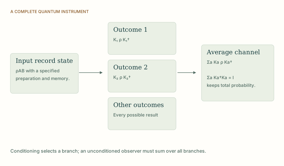
Each local outcome remains equally likely. Indeed the reduced state at either wing is I/2. A distant trace-preserving operation leaves the local reduced state unchanged when its outcome is not conditioned upon. Correlation beyond the Bell bound and no signalling therefore coexist in the same calculation. This is the benchmark for temporal source proposals: a mechanism must reproduce both facts. Explaining only the strong correlation while allowing the remote setting to change a local marginal would describe a different, experimentally constrained theory. ^{[2] [4]}

05A hidden order is a separate issue

A source may generate two output records in a private order while the corresponding detections are spacelike separated in the effective geometry. If that order never changes accessible marginals or joint statistics under a permitted change of foliation, it can remain empirically hidden. If it creates a preferred-frame effect, the theory must predict that effect as a function of physical settings.

Neither option follows from the count of inner levels. Six nested operations are not six loopholes in Bell’s argument and do not by themselves establish Lorentz invariance. A DTT construction must identify the relation between source order, effective causal order and measurable intervention. This is where its distinction between generation and observation can be useful: it allows the underlying organization and the observable influence structure to differ, while requiring a proof of their compatibility. ^{[3] [1]}

06A positive source theorem

A meaningful DTT result would derive a family of nonfactorizing joint completion instruments whose local marginals are independent of remote choices. It should then show why the correlation law has the quantum form rather than an arbitrary no-signalling form. Those are two different restrictions, and both matter.

The source model could also predict a linked multi-time correlation or a memory constraint that ordinary state preparation leaves free. That would make its architecture experimentally informative without requiring superluminal messages. Existing Bell experiments constrain local causal models under their assumptions; they do not uniquely select a Single Monad or any other ontology. The comparison strengthens DTT by making its allowed explanatory route explicit and by turning the no-signalling requirement into a calculation instead of an assertion. ^{[2] [3] [5]}

THE SAME QUESTION, DIFFERENT STARTING POINTS

The comparison at a glance

Continue on SMONAD

• Simultaneity →

  Connects this comparison with the author’s underlying construction.

• The EPR Paradox →

  Connects this comparison with the author’s underlying construction.

• A finite-update cone →

  Connects this comparison with the author’s underlying construction.

• Why light must share the same cone →

  Connects this comparison with the author’s underlying construction.

• SMM/DTT research claim map: results, assumptions and open targets →

  Connects the comparison to the programme’s current statement of results and assumptions.