Electron mass and scale selection: SMM/DTT and Standard Model quantum field theory
Can a temporal spectral mode explain the electron mass without importing the mass through a chosen inner period? This article compares the source-based construction with Standard Model quantum field theory, identifies their strongest point of contact, and works through a concrete example that separates a valid mathematical result from the further physical relation needed to explain observations.
A mass spectrum requires both dimensionless structure and a physical scale. Integer eigenvalues can organize ratios, but converting an eigenvalue into kilograms or electron-volts needs a normalization. A relation such as E=ħω becomes a prediction of electron mass only if the relevant frequency and its coupling to an electron state are fixed independently.
This is the difference between explaining quantization and selecting a measured value. Many systems have equally spaced modes but radically different frequency scales. The electron also has spin, charge and chiral couplings, so assigning its mass to the first mode of a circle does not identify the electron unless the same model supplies those properties. [1][2][3]
02The SMM/DTT contribution
DTT offers an intuitive interpretation of rest energy as persistent inner production associated with an outer matter record. The six nested inner levels may organize a mode whose completion is stable enough to appear as a particle. That view becomes mathematically useful when a source Hamiltonian or spectral operator defines the mode and its observable energy.
An internal circle must be dimensionally specified. If its radius is a length R, a relativistic Kaluza–Klein-like spectrum has a mass scale ħ/(Rc). If the parameter is an inner time T, the corresponding scale is ħ/(Tc²). Confusing these units can hide a fitted scale. The source dynamics must select the radius or period, and show why the electron occupies the indicated mode.
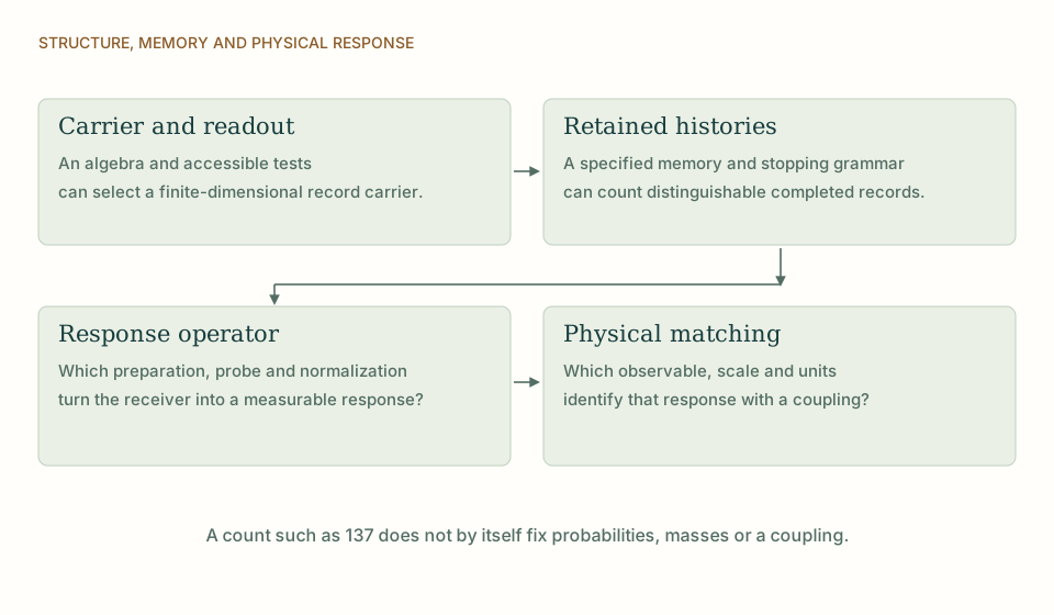
From carrier structure to a measurable response. Representation dimension, a chosen retention grammar, a response operator and physical calibration are separate stages of the constants programme. View full size ↗
03How Standard Model quantum field theory frames the problem
The Standard Model describes matter and nongravitational interactions with quantum fields, internal gauge symmetry and a Higgs sector. Particle representations, coupling constants and several mass parameters are inputs constrained by experiment. Its success makes it the immediate low-energy benchmark for any proposed source theory of matter, while leaving important questions about the origin of those inputs open.
A DTT comparison should therefore distinguish explanation of a parameter from reproduction of a formula that already contains it. A source-derived carrier or completion law would be useful if it restricts representations, couplings or relations among observables. It must still reproduce the field-theoretic meaning of charge, spin, locality and radiative corrections. [1][4]
04Where the mechanisms agree and differ
The Standard Model relates the electron mass to a Yukawa coupling and the Higgs vacuum scale. It explains how a chiral fermion acquires mass consistently with electroweak gauge structure, while the small electron Yukawa coupling remains an empirical parameter. DTT's temporal spectral interpretation is therefore most useful if it explains that small dimensionless ratio or the relevant scale through source dynamics.
A first inner mode does not by itself identify the electron. It must have the correct spin and charge and reproduce the interaction through which its mass is measured. Six nested inner levels can organize a stable completion, but the period in the mode formula remains a free physical input unless selected independently. The worked calculation below demonstrates the circularity clearly: choosing the reduced Compton time reproduces the electron mass because it was calculated from that mass. A strong source result would instead derive a ratio to another independently fixed scale and show that the relation survives radiative corrections. That could supplement the Standard Model mechanism rather than contradict it. The comparison distinguishes an explanation of mass generation from an explanation of the numerical value of one particle's mass. [1][4]
05Worked example: assumptions, calculation and result
Take an internal time coordinate τ with period 2πT. The operator −i∂τ has eigenvalues n/T for periodic functions exp(inτ/T). If physical energy is Eₙ=ħ|n|/T, then mₙ=ħ|n|/(Tc²). The integer spacing follows from the boundary condition, while T remains an input.
For the observed electron rest energy approximately 0.511 MeV, the reduced Compton time ħ/(mₑc²) is about 1.29×10⁻²¹ s. Choosing T equal to this value reproduces the electron mass by construction. A predictive model instead obtains T from another independently fixed quantity or predicts a dimensionless mass ratio. Antiperiodic boundary conditions would shift n to n+1/2, illustrating that the boundary condition also carries physical information. [1][2][3]
ωₙ=n/T; mₙ=ħ|n|/(Tc²). For a length radius R=cT, mₙ=ħ|n|/(Rc).
T is a time and R a length; the circle period is 2πT or circumference 2πR. Periodic versus antiperiodic domains give different spectra.
06An independent operational check
Mass definitions also depend on context. A parameter in a bare Hamiltonian, a pole in a propagator and an effective mass in a medium are related but different quantities. A source spectral eigenvalue must be matched to the mass used in the intended observable. Otherwise a small discrepancy can reflect mismatched definitions rather than a new temporal correction. The electron calculation is most informative when it fixes a free-particle mass relation and then uses that same relation in another setting, such as atomic binding. This provides an independent check that the source mode is a physical particle property and not only an adjustable clock period.
07What follows from the comparison
The useful contribution of a temporal spectral model can be a constrained pattern of masses or a protection principle for a light mode. Absolute scale selection is a separate result. A convincing electron calculation also reproduces its charge and spin and remains stable when interactions renormalize the effective mass. These requirements focus the proposal on physical content rather than a numerical substitution.
THE SAME QUESTION, DIFFERENT STARTING POINTS
The comparison at a glance
Question
SMM/DTT
Standard Model quantum field theory
Starting physical structure
One nonspatial source; six nested inner functional levels produce records accessible through outer completion.
Complex quantum fields in gauge representations, with a Higgs sector and measured parameters.
The central mechanism in this topic
The source must select a dimensionless mass ratio or an independent inner scale.
The Higgs mechanism gives mₑ=yₑv/√2 in natural units, with yₑ an input.
How the claim is made operational
A source-to-record map must define geometry, material response and physical clocks with shared inputs.
A local action, quantum amplitudes, renormalization and comparison with measured observables.
Meaning of agreement
Agreement is a compatibility result; a source-selected relation or fixed residual would add explanatory content.
The stated framework provides a benchmark within its own assumptions and established domain.
KEEP THE CONNECTION
Key ideas
A temporal model is strongest when it explains the small Yukawa ratio and preserves the known interaction structure.
The worked example establishes only the result stated under its explicit assumptions.
Six nested inner levels describe one generative organization; outer time orders accessible completion.
Develops the source construction or operational distinction used in this comparison.
Sources and further reading
References support the comparator and the specific mathematical or interpretive claims indicated. SMM/DTT connections are developed in the analysis above.