


The answer in brief
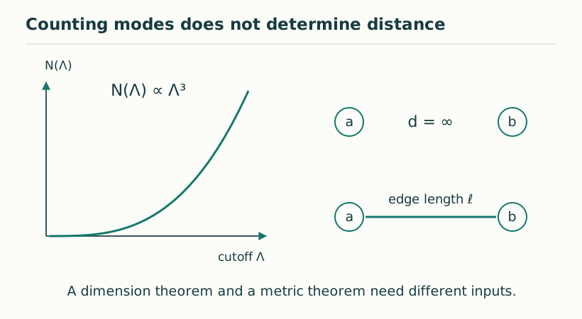
Rank, covering dimension and spectral dimension measure different structures. Their agreement in a physical regime must be demonstrated using independently defined geometry, clocks and probes.
Go to the research challengeDifferent dimension measurements answer different questions
A source construction may contain a rank-three detector, a branching record archive and a diffusion process. Each supports a different dimensional diagnostic. Readout rank counts independent linear components. A covering exponent measures how many distinguishable regions are needed at finer resolution. A spectral dimension measures how a specified return statistic changes with its diffusion parameter.
These quantities can agree in a suitable regime, but agreement is a result to demonstrate. They can also differ without contradiction. In SMM/DTT, the six nested inner levels can organize record refinement while the chosen paired readout has three components. Neither observation alone identifies the dimension measured by every geometric or dynamical probe.
The refinement and dimension guide provides the appropriate starting point: define the records, metric, measurement scale and probe before interpreting an exponent as physical spatial dimension.
Refinement produces an exact scaling dimension
Suppose every record has B distinct children and each refinement reduces the comparison scale by a fixed factor r, with 0<r<1. At depth n there are Nₙ=Bⁿ cylinders and scale ℓₙ=Lrⁿ. The ratio log Nₙ/log(L/ℓₙ) is log B/log(1/r), independent of n.
For an infinite address space with distance determined by the length of the common prefix, these cylinders are the natural metric neighborhoods. Give each depth-n cylinder weight B⁻ⁿ. Its weight is proportional to (ℓₙ/L)ᴰ with D=log B/log(1/r), providing the matching count and measure scaling used to identify the record dimension.
A finite collection of sampled records does not literally acquire a positive Hausdorff dimension by this formula; a finite metric set has dimension zero at sufficiently fine resolution. Its measured slope concerns a finite scale range or an intended infinite refinement limit. Stating that range prevents a finite demonstration from being mistaken for a completed continuum theorem.
The occupation measure is another independent choice
A two-branch construction with contraction one-third has the same cylinder count whether the branch probabilities are equal or unequal. At depth two, equal independent weights give four probabilities of one-quarter. Branch probabilities 3/4 and 1/4 instead give 9/16, 3/16, 3/16 and 1/16. The set of four cylinders and their scales are unchanged.
A probe sampling completed records according to those weights encounters a different statistical geometry. Thus a source proposal should distinguish the number of available regions from their occupation and from the dynamics of motion between them. Changing a sampling measure may affect a measured return law while leaving the underlying covering count fixed.
Three coordinate directions can contain a lower-dimensional set
Take the usual middle-third Cantor construction independently in each of three coordinates. At every stage retain the eight corner subcubes of side one-third. After n stages there are 8ⁿ retained cubes of scale 3⁻ⁿ. The resulting product set has similarity dimension log 8/log 3, approximately 1.893, while its affine span is three-dimensional.
The self-similar dimension statement uses the separation conditions of the construction. The relevant general framework is given by Hutchinson, Fractals and Self-Similarity: for contracting similitudes with the open set condition, the similarity exponent agrees with Hausdorff dimension. The corner-cube example satisfies the needed separation.
This supplies a direct counterexample to the identification of rank with covering dimension. Three available coordinates describe the embedding and independent directions of its affine span. The occupied set is sparse across refinements. A DTT readout should therefore report occupation measure and accessible geometry in addition to its rank.
A finite diffusion probe has a scale-dependent slope
Consider continuous-time diffusion on a four-cycle with graph Laplacian L and unit edge rates. Its Laplacian eigenvalues are 0,2,2,4. The normalized heat trace, also the average return probability, is P(t)=(1+2e⁻²ᵗ+e⁻⁴ᵗ)/4. This is finite for every nonnegative t and tends to 1/4 as the finite graph equilibrates.
The spectral diagnostic is dₛ(t)=−2d log P/d log t. Direct differentiation gives dₛ(t)=8t/(e²ᵗ+1). It approaches zero at both very short and very long times. At t=1/2 it is 4/(e+1), approximately 1.076. The probe has not counted a fractional number of graph coordinates; it has measured a changing logarithmic slope of a finite return law.
A dimensional interpretation requires a scale window and control of finite-size effects. The spectral-dimension article also explains why a proposed return observable must be finite before its slope can be used.
A changed clock can alter a diffusion diagnostic
Suppose a valid return law in an intermediate regime is P(u)=Cu⁻ᵈ/². If operational diffusion time is related deterministically to a measured parameter by u=atᵟ, substitution gives P(t)=Ca⁻ᵈ/²t⁻ᵟᵈ/². Its slope with respect to log t is therefore δd. The underlying record set and its coordinate rank have not changed.
This conditional calculation shows how temporal response can affect a spectral diagnostic. It does not apply automatically to every random clock. In a stochastic model one must average the actual kernel over the clock distribution, check normalization and verify that the return quantity is finite. Singular point probes and finite detector cells can behave differently.
For SMM/DTT, the constructive task is to derive the clock response independently and calculate the chosen diffusion measurement with that response. Fitting both the clock and dimension from one return curve would not establish their proposed physical relation.
Compare several probes on one fixed source
Choose one refinement family and retain its update, readout and calibration. Measure affine rank, cylinder counts, neighborhood growth and a finite return statistic independently. Plot their estimates over a declared scale range and vary detector resolution and graph size. Agreement should remain stable when these auxiliary choices change within the claimed regime.
The deliverable should explain every disagreement. It might arise from a nonuniform measure, an ill-conditioned detector, a finite-volume cutoff, a changing clock law or a genuine structural distinction. A difference is informative once the measured quantities are named precisely.
This comparison gives the dimensional-emergence programme a stronger foundation. The desired physical three-dimensional world involves compatible observation and motion, not only a single attractive exponent. Demonstrating when distinct probes converge to the same geometry would be a meaningful source-level result.
Develop the argument
Questions to take further
- Do covering, detector and diffusion estimates converge over the same controlled scale range?
- Can a change in the clock law explain a changed return slope without changing the underlying spatial readout?
A concrete next step
Compare dimensional probes
Fix one source and refinement family; independently compute rank, neighborhood counts and a finite return observable with calibrated time.
What to share
A reproducible comparison across resolutions, with finite-size effects and every interpretation of dimension stated.
I welcome collaboration with experts in physics, mathematics and philosophy. Get in touch with a question or proposal.