Can a source dynamically select local structure?

A local graph is a result to generate and maintain

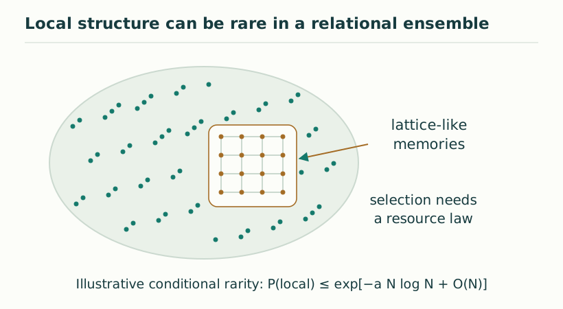
A source can be programmed to produce a lattice, demonstrating that local relations are compatible with a common generative process. Dynamic selection asks a stronger question: why does a suitable neighborhood arise from a class of preparations without storing its full desired arrangement in advance?

The source needs a state space of possible relations, a rule changing those relations and a criterion that favors or stabilizes the intended structures. The state space and criterion are physical assumptions to inspect. A result should show which properties follow from them and which were already encoded by restricting the allowed candidates.

The programmed geometry article identifies this distinction. It creates a positive research path from exact finite construction to selection, stability and the cost of preparing local structure.

A simple degree rule leaves a calculable ambiguity

Consider every simple undirected graph on six labeled vertices. There are fifteen possible edges and therefore 2¹⁵=32,768 graphs. Give each graph the nonnegative energy E(G)=Σᵥ(deg(v)−2)². Zero-energy graphs have degree two at every vertex, so each connected component is a cycle of length at least three.

With six vertices, a zero-energy graph is either one six-cycle or two disjoint triangles. There are (6−1)!/2=60 labeled six-cycles. There are ½ times the number of three-element subsets of six vertices, namely ten, ways to divide the vertices into two unordered triangles. Thus the rule selects seventy ground-state graphs, and ten are disconnected.

The degree preference is doing real work: it excludes nearly all possible graphs. Yet it does not enforce connectedness. Under equal weighting of its zero-energy states, the probability of a connected six-cycle is 60/70=6/7. This is a derived probability for the explicitly chosen finite ensemble, not an estimate of how likely physical space is to exist.

A stronger criterion should disclose what it adds

Add λ(c(G)−1) to the energy, where λ>0 and c(G) is the number of connected components. Among the zero-degree-error graphs, a single cycle has no extra cost while two triangles have cost λ. Since all terms are nonnegative and six-cycles attain zero, the global ground states of the new energy are exactly the labeled six-cycles.

This is an exact selection statement, but the connected-component term is global. A physical source must explain how its update evaluates or enforces that preference. Computing c(G) through a hidden unrestricted controller can introduce memory and communication unavailable to the proposed local mechanism. A scalar objective function is not yet its autonomous realization.

A more demanding construction could use local auxiliary records that certify connectedness through a retained spanning structure. The preparation and verification of those records would enter the source budget. The six nested inner roles might organize such work, but a proof must include the information each role receives and preserves.

A decreasing cost does not guarantee the desired outcome

One possible update toggles a candidate edge and accepts the move when the energy decreases. This rule cannot increase the objective, but it may stop at a local minimum with positive energy. A convergence theorem must rule out such traps or describe the additional moves needed to escape them. Running one successful example does not prove convergence from every allowed preparation.

A finite stochastic alternative allows all edge toggles and accepts an energy-increasing move with a specified nonzero probability. With symmetric proposals and acceptance min(1,exp(−βΔE)), the weights proportional to exp(−βE) satisfy detailed balance. For neighboring graphs, multiplying the transition probability by its starting weight gives the same value in both directions. This proves stationarity of that distribution.

Stationarity does not provide a useful convergence time or guarantee a ground state at finite β. Those require further bounds. Moreover β, the proposal rule and the physical origin of its randomness remain inputs. The finite calculation is valuable because each ingredient and its limited conclusion can be checked independently.

Selected adjacency must constrain later dynamics

Even a perfectly selected cycle fails as a physical locality model if later operations can swap arbitrary distant vertices. Add matter registers and require each transport step to use retained adjacent ports. The neighborhood selection theorem and the support theorem then address different parts of the same source process.

Perturbing one edge can create a shortcut that substantially changes long-distance routes. Stability should therefore bound useful quantities such as shortest-path distortion, the size of affected neighborhoods and leakage of influence outside the intended cone. A small average degree error can coexist with a damaging long edge, so the energy chosen above is not a complete stability diagnostic.

For a finite comparison, delete one cycle edge and add a chord. Recompute all pairwise distances and the propagation support of a localized excitation. The resulting changes make the geometric consequences of a relational error explicit and suggest which correction mechanism the source would need.

Move from a target energy to a source mechanism

The immediate research challenge is an autonomous implementation of a modest selection criterion. Specify a finite relational state space, allowed initial preparations, auxiliary memory and update duration. Prove which graph property is eventually reached, how often failure occurs if the mechanism is stochastic, and how much work is needed to verify completion.

Then couple transport through the resulting graph without adding a hidden channel. The strongest useful finite result would connect formation, verification and later local influence under one resource budget. It would clarify whether the source genuinely selects the neighborhood or only transfers a prearranged neighborhood from an external description.

A cycle is intentionally a small target. Selecting a stable three-dimensional neighborhood, an isotropic metric and compatible material clocks requires further structure. The finite example turns that ambition into a sequence of measurable and provable tasks that collaborators can extend.

Continue reading

• Why local geometry can be statistically rare →
• The information cost of preparing locality →
• Programmed geometry and spontaneous selection →
• Open problem: selecting and preserving spatial locality →

Read this discussion as part of a path

• How does generation become space? →