


Assumptions, results and research status
Exact results for the supplied scalar, nonrelativistic Coulomb Hamiltonian; its DTT source derivation is a separate target.
Assumptions
- The state space is L²(ℝ³) with the usual probability measure and a normalized scalar wavefunction.
- The Hamiltonian is H = −D∇² − C/r with D > 0, C > 0, and separation threshold zero.
- Spin, radiation, finite nuclear size, and external fields are omitted from this leading model.
Results
- The unique scalar ground state is exp(−r/a)/√(πa³), with a = 2D/C and E₁ = −C²/(4D).
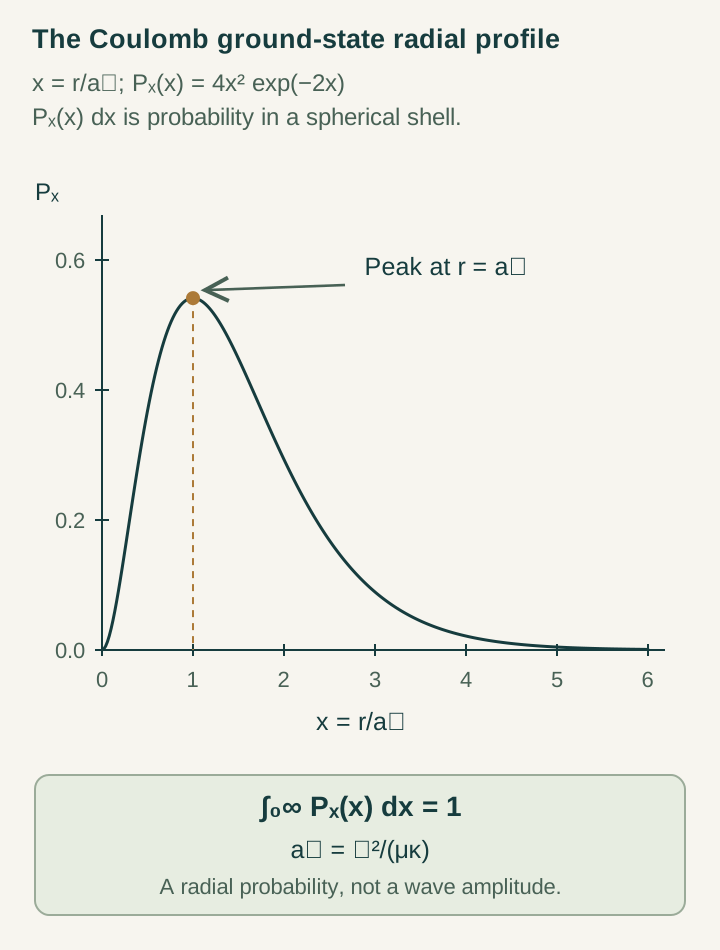
- Its radial density peaks at a, while its mean separation is 3a/2 and only about 32.3% of its probability lies inside a.
- Kinetic energy, potential energy, radial moments, and momentum variance follow from the same normalized state.
Open question: Can the temporal source construction recover this common operator and probability measure, including its coefficients, rather than impose the ground-state profile as an input?
Fix the problem and its energy threshold
Let r = |x| be the relative separation of the two constituents. Supply positive coefficients D and C and the quadratic energy form:
∫|ψ|2d3x = 1
The natural form domain is H1(ℝ3): square-integrable functions with square-integrable first weak derivatives. The Coulomb singularity is controlled by the three-dimensional Hardy inequality and Cauchy–Schwarz, which give ∫|ψ|2/r ≤ 2‖ψ‖2‖∇ψ‖2. This makes the potential arbitrarily small relative to the kinetic form, at the cost of an additional finite constant.
The form consequently defines the usual lower-bounded self-adjoint Coulomb Hamiltonian. Since the potential tends to zero at infinite separation, the separated-particle threshold is zero. A negative normalizable eigenstate represents binding relative to that threshold.
These are the effective inputs behind Paper 12’s conditional reconstruction. The calculation below establishes their consequences without claiming that the temporal source construction has already produced them. [Paper 12]
Find the length by direct substitution
Try ψ(r) = Ne−r/a, with positive length a and normalization N still unknown. For a radial function away from the origin, ∇2ψ = ψ″ + 2ψ′/r. Substitution gives:
Hψ = [−D/a2 + (2D/a − C)/r]ψ
An eigenvalue must not depend on r. The inverse-distance coefficient therefore vanishes precisely when a = 2D/C. The remaining term is constant, yielding E1 = −D/a2 = −C2/(4D).
The identity also has the appropriate weak meaning at the origin. Unlike 1/r, this exponential has no finite point-source flux through a sphere shrinking to zero, so its Laplacian does not acquire a delta function there.
At this stage we have an eigenfunction and its eigenvalue. We still need to exclude a state with lower energy. That is the role of the next step; choosing a plausible shape and minimizing its scale would not by itself settle the global problem.
Prove the lower bound for every state
Write r̂ = x/r and complete the square. The cross term is a−1r̂·∇|ψ|2. Integration by parts uses ∇·r̂ = 2/r in three dimensions, with no point delta term. For a = 2D/C:
= q[ψ] + (D/a2)‖ψ‖22 ≥ 0
The identity is first established for smooth test functions and extended to the form domain. Every normalized admissible state therefore has q[ψ] ≥ −D/a2. The exponential makes the square vanish because ∇ψ = −r̂ψ/a. It attains the universal lower bound and is a ground state.
Equality also fixes its spatial shape. Multiplying the equality equation by er/a shows that the weak gradient of er/aψ is zero. The product is constant almost everywhere on the connected space. Thus the scalar ground eigenspace is one-dimensional, apart from an overall complex amplitude.
Additional internal spin labels would enlarge the supplied state space. They do not alter this uniqueness statement for the scalar spatial problem.
Normalize the state and its probability measure
Spherical integration gives 1 = 4π|N|2∫0∞r2e−2r/adr. Using ∫0∞rke−λrdr = k!/λk+1 for a nonnegative integer k, the radial integral is a3/4. A convenient phase convention gives:
P(r) = 4r2e−2r/a/a3
The spatial probability density |ψ1|2 is largest at the origin. The radial density P(r) includes the volume of a spherical shell and peaks at r = a. These describe different measurements, so their different maxima are expected.
Writing x = R/a, the probability inside radius R is:
For example, F(a) ≈ 0.3233, F(2a) ≈ 0.7619, and F(3a) ≈ 0.9380. The characteristic radius is neither a hard boundary nor a circular trajectory. Explore these distinctions in the probability explorer.
Calculate independent checks from the same state
The normalized radial distribution determines the moments without additional fitting. Direct integration gives ⟨1/r⟩ = 1/a, ⟨r⟩ = 3a/2, and ⟨r2⟩ = 3a2. The radial variance is therefore 3a2/4. The mean separation and the most probable radial separation are different even in this simplest atomic state.
Since |∇ψ1|2 = |ψ1|2/a2, the kinetic and potential expectations are:
E1 = T + V = −D/a2
2T + V = 0
The momentum second moment is ⟨p2⟩ = ħ2/a2. It is nonzero although a real ground-state wavefunction has zero probability current. Momentum variance is not a directed orbit velocity.
These checks make the ground state a strong reconstruction target. Matching its energy alone is less restrictive than recovering its radial distribution, gradient energy, and moments from the same retained probability rule.
Worked example: changing the trial radius
Normalize an exponential with an arbitrary length b and evaluate its energy. Set a = 2D/C and B = D/a2. The result is:
x = b/a: E(b)/B = x−2 − 2x−1
E(b)/B + 1 = (x−1 − 1)2
The optimum is x = 1. A trial state twice as broad gives E/B = −3/4, while one half as broad gives E/B = 0. The narrow state pays a large gradient-energy cost; the broad state loses attraction. At arbitrarily large b, the energy approaches the separation threshold from below.
This curve helps explain the selected scale, but the global square-completion argument is what establishes the exact minimum over all admissible states. The existing energy-balance demo illustrates the same family.
In consistent model units D = 1/2 and C = 1, the results are a = 1, E1 = −1/2, T = 1/2, and V = −1. These are mathematical benchmarks independent of any measured value of alpha.
Attach the reduced-mass physical dictionary
For electron and proton masses me and mp, let μ = memp/(me+mp). The standard electromagnetic identification supplies D = ħ2/(2μ) and C = αħc. Then:
E1 = −μc2α2/2
The conventional Bohr radius a0 uses the electron mass, whereas this two-body relative coordinate uses μ. Consequently aμ = a0(1 + me/mp). The finite proton mass slightly enlarges the relative atomic scale and reduces the leading binding magnitude compared with an infinitely massive nucleus. Paper 12 retains this distinction. [Paper 12]
A constants-based numerical evaluation should identify its reference data and approximation. The interactive scales explorer links those inputs to the quantities derived here. More precise hydrogen energies need relativistic, radiative, recoil, and nuclear-structure contributions beyond this Hamiltonian.
Connect the result to temporal persistence
Under the supplied Schrödinger evolution, the ground state acquires a uniform phase e−iE₁t/ħ while its position probability stays fixed. That is a precise effective model of persistent atomic organization. It does not by itself explain how a general initial state becomes this ground state.
A physical account of relaxation needs additional interactions or a specified preparation instrument. The distinction matters for SMM/DTT: a completed state and the autonomous process that prepares its record are separate pieces of the construction. The completion example shows how a probability and a state change can be defined explicitly.
The source-level target is now concrete. Derive the kinetic coefficient, the attractive response, the continuum measure, and the clock normalization together; then recover the bound, normalized profile, and moment relations as consequences. Paper 21 describes hydrogen as a point where these independent responsibilities converge. [Paper 21]
Continue to quantum numbers and the full leading spectrum to see how the same Hamiltonian also determines the higher bound states.
Continue reading
Sources for this guide
Source manuscripts, version notes, and standard references are listed in the reference library.