
For H=−DΔ−C/r, with positive D and C, square completion gives a=2D/C and E₁=−C²/(4D). Normalization, radial moments and the kinetic–potential balance follow from the same state.
Inputs: state space, coefficients and threshold
Let r=|x| be the relative separation of two constituents in three-dimensional Euclidean space. States belong to L²(ℝ³), with normalization ∫|ψ|²d³x=1. Supply two positive coefficients D and C and the energy form q[ψ]=D∫|∇ψ|²d³x−C∫|ψ|²/r d³x on the Sobolev space H¹(ℝ³). The operator H=−DΔ−C/r means the self-adjoint realization associated with this closed, lower-bounded form.
The dimensions are [D]=energy×length² and [C]=energy×length. The potential tends to zero at infinite separation, fixing the separated-particle threshold at zero. Negative energy can therefore signal binding in this model. These inputs specify geometry, the probability rule and an attractive interaction; they are the effective ingredients that a source-level SMM/DTT construction must eventually produce.
The Coulomb singularity is controlled, rather than omitted. The three-dimensional Hardy inequality and Cauchy–Schwarz give ∫|ψ|²/r≤2‖ψ‖₂‖∇ψ‖₂. Consequently the potential is infinitesimally bounded relative to the kinetic form: an arbitrarily small positive multiple of ‖∇ψ‖₂², plus a finite multiple of ‖ψ‖₂², bounds its magnitude.
Step 1: find a candidate by direct substitution
Try a radial exponential ψ=N exp(−r/a), where a is a positive length and N is to be fixed. For r>0, the radial Laplacian is f″+2f′/r. The first and second derivatives of this exponential are −ψ/a and ψ/a², respectively.
Hψ=[−D/a²+(2D/a−C)/r]ψ
An eigenvalue must be independent of position. Cancel the coefficient of 1/r by setting a=2D/C. The remaining coefficient gives E₁=−D/a²=−C²/(4D). Both the length and energy therefore come from the same cancellation. The calculation holds weakly across the origin; the radial flux through a sphere of shrinking radius tends to zero, so no point-source delta term is introduced by this exponential.
This step finds an eigenfunction. It has not yet excluded a different state of lower energy. A variational estimate alone would likewise give only an upper bound on the ground energy.
Step 2: prove a global bound by completing the square
Write r̂=x/r and expand |∇ψ+r̂ψ/a|². The cross term is a⁻¹r̂·∇|ψ|². Integration by parts replaces its integral by −a⁻¹∫(∇·r̂)|ψ|². In three dimensions ∇·r̂=2/r, including its distributional meaning; its flux at the origin vanishes. Start with smooth test functions and extend the identity by continuity to H¹.
=D∫|∇ψ|²d³x−(2D/a)∫|ψ|²/r d³x+(D/a²)‖ψ‖₂²
=q[ψ]+(D/a²)‖ψ‖₂²≥0
With a=2D/C, every normalized state satisfies q[ψ]≥−D/a². The exponential has ∇ψ=−r̂ψ/a and makes the square vanish. It therefore attains the universal lower bound and is a ground state. This is stronger than optimizing a guessed radius within a restricted family.
Equality also determines the spatial shape. The equation ∇ψ=−r̂ψ/a implies that exp(r/a)ψ is constant almost everywhere. Thus the spinless scalar ground eigenspace is one-dimensional, apart from its constant complex amplitude. Additional internal labels require a separately specified state space.
Step 3: normalize the state and its radial measure
Spherical integration gives 1=4π|N|²∫₀∞r² exp(−2r/a)dr. The elementary identity ∫₀∞rⁿ exp(−λr)dr=n!/λⁿ, for nonnegative integer n and λ>0, yields an integral a³/4. Choosing a positive overall amplitude gives:
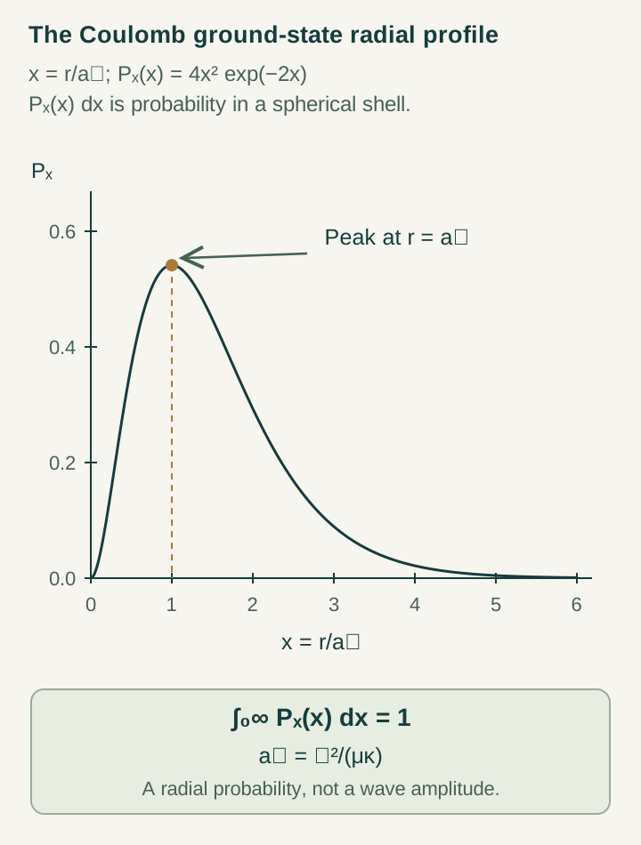
P(r)=4r²exp(−2r/a)/a³
x=r/a: P(r)dr=4x²exp(−2x)dx
The probability density per unit volume is |ψ₁|². The radial probability P includes the volume of a spherical shell. These are different quantities: the former is largest at the origin, while the latter peaks at r=a. A peak in P describes a most probable radial interval, not a sharply defined circular electron orbit.
Open the full-size diagram →
Step 4: check moments and the energy balance
The same integrals give ⟨1/r⟩=1/a, ⟨r⟩=3a/2 and ⟨r²⟩=3a². Hence the radial variance is 3a²/4. The finite spread verifies localization while showing that the atom is not concentrated on a thin shell. In particular, the mean radius and the peak radius are different even for this simplest state.
Because |∇ψ₁|²=|ψ₁|²/a², the kinetic expectation is T=D/a². The potential expectation is V=−C/a=−2D/a². Their sum is E₁=−D/a², agreeing with substitution and with the global bound.
These equalities provide linked checks for an approximation or a discrete source model. Matching only the energy would leave the radial measure and momentum scale untested. Matching the energy, moments and kinetic–potential balance places much stronger restrictions on the generated state.
Step 5: separate a variational curve from the exact proof
Normalize exp(−r/b) for an arbitrary positive trial length b. Its expectation is E(b)=D/b²−C/b. Set x=b/a and E*=D/a². Then E(b)/E*=x⁻²−2x⁻¹, and E(b)/E*+1=(x⁻¹−1)². The minimum in this family occurs at x=1.
The hydrogen energy demonstration plots this exact family. The curve explains the balance: small radii increase the gradient cost faster than the attraction, while large radii approach the separation threshold. Its minimum agrees with the global proof, which is what establishes that no state outside the family does better.
For D=1/2 and C=1 in consistent model units, a=1, E₁=−1/2, T=1/2 and V=−1. This example supplies convenient benchmarks without importing an empirical value of the electromagnetic coupling.
Step 6: attach the physical dictionary
For constituent masses m and M, the relative reduced mass is μ=mM/(m+M). Supply an action scale ħ and set D=ħ²/(2μ), C=għc. The exact formulas become a=ħ/(μcg) and E₁=−μc²g²/2. The interaction strength g is dimensionless. Electromagnetic identification sets g=α after the interaction and unit conventions have been fixed.
Every positive g gives a normalized ground state, with size proportional to g⁻¹ and binding magnitude proportional to g². Binding by itself does not select g. A count of source records can only determine it after a physical response law connects that count to C relative to the same ħ and c used in matter propagation.
Result: a precise target for temporal completion
Under iħ∂ₜψ=Hψ, the ground state acquires the phase exp(−iE₁t/ħ), while its probability density remains fixed. This is a concrete example of persistent recorded structure with evolving phase. Calling it a completed atomic mode is useful when the meaning of completion includes this supplied dynamics; the stationary form alone does not prove a preparation mechanism.
The SMM/DTT programme asks one source, with six nested inner roles and outer completion, to generate the continuum operator, its coefficients and its retained probability rule. The lower bound, normalized profile, moments and speed identity are then simultaneous consequences to recover. A further model is needed for relaxation into this mode, spin, radiation and corrections to the Coulomb approximation.
Continue with the articles
- Why the Coulomb law requires a continuum input
Explain the additional three-dimensional Poisson assumption that yields a one-over-distance potential. Separate this matching step from the finite record-graph construction.
- A normalizable hydrogen-like ground state
Introduce the lower-bound and bound-state results of the effective model. Explain how the supplied kinetic and potential rules produce a meaningful atomic test case.
- Why binding does not fix the coupling
Introduce the dilation argument showing that a family of positive couplings remains compatible with binding and completion. Identify the extra source-selection law needed to obtain a specific interaction strength.
- Freeze parameters before predicting spectroscopy
Explain the post-freeze strategy proposed for atomic observables. A spectroscopy comparison becomes informative when its coefficients are fixed without using the same transitions as targets.