
The normalized Coulomb ground state gives √⟨p²⟩/μ=cg. After electromagnetic matching g=α, this is a relative RMS speed; the electron speed in the centre-of-mass frame has the additional factor μ/mₑ.
Inputs: one Hamiltonian and one velocity observable
Take the relative Hamiltonian H=p²/(2μ)−C/r on L²(ℝ³), with p=−iħ∇, reduced mass μ>0 and attractive coefficient C>0. Define the dimensionless interaction parameter g=C/(ħc), where c is the independently supplied reference speed. The Coulomb ground-state derivation gives a=ħ²/(μC)=ħ/(μcg) and E₁=−μc²g²/2.
The relative velocity operator is v= p/μ. It follows from the Heisenberg equation (i/ħ)[H,x]=p/μ because the potential commutes with position. This fixes which observable is meant before the speed is calculated. Its RMS magnitude is vrel,rms=√⟨v·v⟩=√⟨p²⟩/μ.
These are nonrelativistic definitions. The resulting relation applies within this effective model and is accurate as a physical approximation where relativistic and other corrections are controlled. A small value of g makes the characteristic ground-state speed small compared with c; it does not impose a hard upper bound on every momentum measurement in the Schrödinger model.
Step 1: calculate the momentum moment directly
The normalized ground state is ψ₁=exp(−r/a)/√(πa³). Its weak gradient is ∇ψ₁=−r̂ψ₁/a. The quadratic-form definition of the momentum second moment gives:
vrel,rms=ħ/(μa)=C/ħ=cg
No circular orbit or uncertainty estimate entered this equality. It follows by integrating a normalized eigenstate using the already defined operator. The same a fixes both the radial shape and momentum scale, so a model that reproduces only one of them has not reproduced the full atomic state.
Spherical symmetry gives ⟨pₓ²⟩=⟨pᵧ²⟩=⟨p_z²⟩=ħ²/(3a²). The RMS velocity of one Cartesian component is cg/√3. This illustrates why the observable must be specified: the RMS magnitude and the RMS value along one direction are not equal.
Step 2: reconcile nonzero RMS speed with zero current
Choose the spatial ground wavefunction real. Its probability current is j=(ħ/μ)Im(ψ*∇ψ)=0, and ⟨p⟩=0. The time-dependent global phase does not change either conclusion. Nevertheless ⟨p²⟩ is positive. A zero mean vector does not imply that the vector has zero variance.
Thus the formula does not assign a hidden circular trajectory or a circulation period to an electron. It specifies a quantum momentum statistic. Mean speed ⟨|p|⟩/μ is another possible statistic and should not be substituted for √⟨p²⟩/μ without a separate calculation.
For SMM/DTT, an interpretation in terms of discrete source advances must explain how the retained velocity observable is built and why it has this moment. Merely calling a source delay an electron speed would leave the operational identification unproved.
Step 3: derive the independent virial check
For a normalized bound eigenstate ψ, consider the normalized dilation ψλ(x)=λ3/2ψ(λx). A change of variables shows T(λ)=λ²T and V(λ)=λV for a Coulomb potential. Hence the expectation is E(λ)=λ²T+λV.
An exact eigenstate is stationary under differentiable normalized variations. Differentiating at λ=1 gives 2T+V=0. This follows from the variational stationarity of an eigenstate, whether or not that state is the ground state; the required finite moments and dilation regularity hold for Coulomb bound states.
⟨p²⟩=−2μE
Inserting E₁=−μc²g²/2 reproduces ⟨p²⟩=μ²c²g² and therefore vrel,rms=cg. The direct gradient calculation and the dilation argument agree while testing different parts of the construction.
Step 4: extend the relation to bound energy levels
The full Coulomb spectral problem gives En=−μc²g²/(2n²), where n is a positive integer. Using that spectrum as an additional known result, the same virial identity yields vrel,rms/c=g/n for each bound energy eigenstate. This step derives the speed from the spectrum; it is not a separate derivation of the entire spectrum.
The squared speed scales as n⁻², just like the binding-energy magnitude. At n=2, RMS speed is half its ground-state value and binding energy is one quarter. Different angular momentum states at the same n can have different spatial distributions while sharing this total momentum second moment.
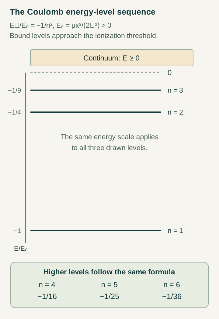
Open the full-size diagram →
Step 5: distinguish the electron and relative motions
Let xₑ and xN be electron and nuclear positions, r=xₑ−xN, and R=(mₑxₑ+MxN)/(mₑ+M). Then xₑ=R+[M/(mₑ+M)]r. In the centre-of-mass frame the momenta are p and −p; the electron velocity is p/mₑ, while relative velocity is p/μ with μ=mₑM/(mₑ+M).
vN,rms/c=(μ/M)g/n
Only the infinitely heavy nucleus limit makes the electron ratio equal to g/n. For equal constituent masses, each centre-of-mass RMS speed is half the relative RMS speed. The two velocity vectors are anticorrelated, so the relative second moment must be formed before taking its square root.
At fixed coupling, changing nuclear mass changes a and E through μ, whereas the relative RMS ratio stays g/n. The electron ratio still changes through μ/mₑ. These distinct mass dependences give a useful consistency requirement for a proposed source model.
Step 6: evaluate an ideal 137 example
Choose g₀=1/137 as an illustrative ideal-model input and n=1. Then vrel,rms/c=1/137≈0.00729927 and |E₁|/(μc²)=1/(2×137²)≈0.0000266397. For a model nucleus with M=2000mₑ, the electron ratio is 2000/(2001×137)≈0.00729562.
These numbers follow from chosen parameters, without using an empirical value of alpha. The atomic length is a=137ħ/(μc). Consequently the dimensionless products |E₁|a/(ħc)=1/(2×137) and μavrel,rms/ħ=1 are linked checks of the same model. They cannot be adjusted independently while keeping the declared Hamiltonian.
The structural integer 137, its reciprocal as an ideal coupling label, and a measured electromagnetic coupling remain distinct stages of the research argument. A correction from one to another must be calculated from a specified dynamics and observable.
Result: what would make this a source prediction?
Electromagnetic matching sets C=e²/(4πε₀) in SI units and defines α=C/(ħc). The exact ground-state identity then reads vrel,rms/c=α. It checks the coupling through an atomic consequence, but it does not select alpha: every positive g in the supplied family satisfies its corresponding identity.
A noncircular SMM/DTT route must fix C/(ħc) upstream, using one source dynamics for matter propagation, mediator response, clock calibration and action normalization. The six nested inner roles organize generation; outer completion defines which records and clock readings are available. Neither role counting nor bound-state existence alone fixes the normalized response.
Once that common dynamics selects an ideal g₀, hydrogen supplies several consequences together: radius, binding energy, relative momentum variance and level ratios. Calculated spin, holonomy, recoil and radiative contributions could then extend the comparison. This is the constructive value of the speed identity: it makes the required agreement between source assumptions and atomic observables explicit.
Continue with the articles
- A normalizable hydrogen-like ground state
Introduce the lower-bound and bound-state results of the effective model. Explain how the supplied kinetic and potential rules produce a meaningful atomic test case.
- Why binding does not fix the coupling
Introduce the dilation argument showing that a family of positive couplings remains compatible with binding and completion. Identify the extra source-selection law needed to obtain a specific interaction strength.
- Freeze parameters before predicting spectroscopy
Explain the post-freeze strategy proposed for atomic observables. A spectroscopy comparison becomes informative when its coefficients are fixed without using the same transitions as targets.
- Hydrogen and deuterium as complementary probes
A proposed isotope-comparison article within the differential-test program. Identify which effects are shared and which require separate mass and nuclear inputs before interpreting a residual.
- Designing an overconstrained atomic test
Turn the skeleton draft’s research direction into a practical analysis plan. Require more independent observables than fitted parameters and predeclare the cross-state prediction rules.