
Successive pictures provide displacements; a physical account also needs a clock, lawful transport, and an observer able to retain comparisons.
Recognize a pattern before explaining its movement
A row of lamps can produce a moving bright spot even though each lamp remains fixed. The changing pattern and the material components answer different questions about what moves. This familiar example makes room for a process-based account of motion without deciding that every physical object is a lamp-like appearance.
Time Chest uses related questions to approach generation and manifestation. In SMM, a persistent moving object is something the common source must organize. DTT separates the work involved in forming a configuration from its completed availability. The task is to explain why successive available configurations belong to one lawful trajectory, including the records that let an observer recognize it.
Give four pictures a measurable speed
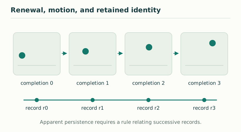
Place a marker at positions zero, two, four, and six centimetres in four successive records. Give those records clock readings zero, one half, one, and one and a half seconds. Each displacement is two centimetres and each elapsed interval is one half second, so the average speed is four centimetres per second.
If the same pictures instead arrive one second apart, their speed is two centimetres per second. Images alone therefore do not fix motion. The comparison also presupposes a ruler convention and a rule identifying the later marker as the continuation of the earlier one.
Write a rule that connects the records
A minimal update is xₙ₊₁=xₙ+vδ and τₙ₊₁=τₙ+δ, with a positive fixed interval δ. Iterating gives xₙ=x₀+vnδ and τₙ=τ₀+nδ. Eliminating n produces xₙ=x₀+v(τₙ−τ₀). This is an exact straight-motion law at the sampled records.
The calculation establishes compatibility once v and δ are supplied. It does not explain their physical values. A stronger SMM model would derive a relation between transport and clock response from one source dynamics. Assigning the two updates to one controller only becomes explanatory when their allowed coefficients are jointly constrained.
A still picture can hide movement
Consider a pointer on a circular dial sampled once each second. A pointer that turns one full revolution per second appears at the same position in every sample. So does a stationary pointer. If the allowed observations are only those samples, the two histories cannot be distinguished from the recorded angles.
Sampling halfway between the original readings separates these particular possibilities: the rotating pointer is opposite its starting point, while the stationary one remains there. Even this enlarged schedule leaves other sufficiently fast motions possible unless additional dynamics or bounds are supplied. The lesson is practical: an observation procedure determines which differences the record can reveal. Smooth or stationary appearance alone does not uniquely reconstruct the hidden process.
A local update gives a limited propagation statement
Now suppose a marker may move by at most one lattice edge during each completed step, and each edge has length ℓ. After N steps its graph displacement is at most N edges. If a calibrated clock advances δ per step, the corresponding average propagation bound is ℓ/δ.
This finite model has a useful causal restriction because an update cannot cross arbitrarily many edges at once. It does not yet establish the light cone of special relativity. A lattice has its own distance rule and preferred structure; different matter and clock sectors may obey different updates. Recovering a common relativistic geometry requires additional transformation, continuum, and universality results.
Separate the source’s work from the object’s route
In the nested DTT picture, six inner roles prepare a readout and outer completion makes it available. A source cursor might visit many internal addresses during that preparation. Its private address sequence is not automatically the path followed by a particle in the completed geometry.
This distinction matters when a counter changes several digits at a carry. Its readout can jump even though a separately defined physical transport operation remains local. A coherent construction identifies which operations build the archive and which move observable patterns through it. It also includes the internal observer’s memory; an external cinema viewer cannot supply the clock and continuity for an entire universe.
Turn the moving picture into a comparison
Use the four-position example to write two predictions before changing the sampling interval. A fixed physical velocity predicts proportional displacement changes; a fixed displacement-per-frame rule may predict a different result if the clock response changes independently. Specifying the intervention exposes what the model actually holds constant.
Continue with A62 for the movie analogy, A67 for discrete and continuous descriptions, and A126 for nested readout. The goal is a complete relation among source update, retained identity, position measurement, and clock reading. Once those relations are stated, apparent motion becomes a calculable outcome rather than a consequence assumed from the picture.
Continue with the articles
- Creation Scenario: the World as a Movie
Use the world-as-a-movie analogy to introduce repeated generation and apparent persistence. Ask what must link frames for the analogy to describe motion, memory, and coherent interaction.
- Discreteness and Continuousness
Explore how discrete records and continuous mathematical evolution can coexist. Introduce the idea that different descriptions may concern different levels or observables rather than competing pictures of one variable.
- The Principle of Ever-renewed Creation
Introduce ever-renewed creation as a central motivation of the Single Monad Model. Ask how the idea might be expressed through histories, completed records, and observable persistence.
- The Cosmic Computer
Develop the cosmic-computer analogy as a way to discuss ordered generation and observable output. Clarify which aspects are metaphorical and which require an explicit computational model.
- Six inner stages and one publication interface
Explain the hierarchy of readout ranks 1, 1, 2, 2, 3, 3 followed by completion. These are nested functional roles rather than six independently readable temporal coordinates.
- A finite-update cone
Introduce the bound relating horizontal displacement to temporal projection in the limiting-speed draft. Explain that the finite-update inequality is a stated geometric assumption.
- Why light must share the same cone
Examine the additional assumption that electromagnetic dynamics inherit the constructed null geometry. A limiting cone in one sector does not automatically establish universal propagation across all fields.
- Reading Volume IV: Time Chest
A reading guide centered on the volume’s particle–wave and temporal-confinement themes, with questions for a later illustrated expansion.