Spacetime discreteness and continuum limits: SMM/DTT and Causal dynamical triangulations
How can discrete production yield continuous motion, and which microscopic details remain visible after refinement? This article compares the source-based construction with Causal dynamical triangulations, identifies their strongest point of contact, and works through a concrete example that separates a valid mathematical result from the further physical relation needed to explain observations.
A continuum limit is a relationship among a family of models, not a visual impression that the cells look small. The lattice spacing or update interval changes while specified physical quantities remain fixed. Correlation functions, distances and propagation laws must converge in an identified regime. A large but fixed network may approximate a continuum for some experiments while failing badly for others.
This matters because different ways of shrinking the same grid produce different physics. Holding the jump probability fixed while changing the waiting time can lead to diffusion, ballistic propagation or a frozen system. The microscopic update and the unit conversion jointly determine the limit. Merely declaring the inner tick very short leaves that relationship unspecified. [1][2][3]
02The SMM/DTT contribution
DTT gives continuity a natural explanatory setting: outer observation reads an accumulated sequence of completed inner processes. The six inner levels are nested operations in this production, not separate continuous axes. A coarse outer observer may be insensitive to individual internal operations and respond only to stable collective correlations.
That interpretation becomes constructive when the source update supplies a refinement rule and a physical resource budget. A faster update cannot be obtained at zero cost merely by relabeling the step number. Clock resolution, interaction strength and retained memory determine which limit is physically meaningful. This is also why a mathematical continuum limit and a realizable infinite-speed computational process must remain distinct.
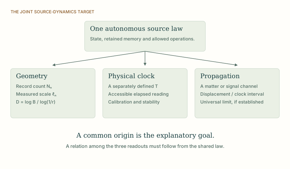
Geometry, clocks and propagation as independent readouts. A single source model should explain the relation between separately defined measurements. Sharing a diagram does not impose that relation. View full size ↗
03How Causal dynamical triangulations frames the problem
Causal dynamical triangulations defines a sum over discretized geometries with a specified causal organization and action. Macroscopic behavior is studied through ensembles and scaling, rather than by treating one fixed triangulation as the final spacetime. Diffusion-based dimension is one useful probe of the generated ensemble. Its numerical behavior is a result inside the model.
The comparison with DTT concerns how a regulated construction produces an extended geometry with stable large-scale observables. A nested inner process is not a triangulation time coordinate, and a computational update used to sample an ensemble is not an observer's clock. Distinguishing these roles is essential when interpreting emergent temporal and spatial behavior. [1]
04Where the mechanisms agree and differ
CDT is a direct comparison for the meaning of a controlled continuum limit. Its geometric building blocks carry a regulator scale, while the large-scale behavior is investigated through an ensemble and its phase structure. DTT would need an analogous family of source models if it claims that discrete generation becomes continuous spacetime in a mathematically defined limit.
A fixed source with an extremely fast update may approximate selected observations, but that is different from proving convergence under refinement. The six nested inner levels can remain structurally fixed while internal resolution changes, allowing a clean separation between functional architecture and regulator size. The example below shows why the accompanying clock scaling must be stated: different choices lead to different continuum equations. A useful DTT contribution would be a universality argument explaining which completion details cease to matter and which determine the effective metric and speed. CDT also cautions against treating a numerical sampling step as physical time. If source dynamics is claimed to be physically autonomous, its actual clock observable must be defined separately from any algorithm used to calculate its ensemble. This distinction turns a vague continuity claim into a reproducible construction. [1]
05Worked example: assumptions, calculation and result
For a symmetric one-dimensional random walk, each step changes position by ±a with equal probability. After n steps, ⟨x⟩=0 and ⟨x²⟩=na². Setting physical time t=nδt gives ⟨x²⟩=(a²/δt)t. A nontrivial diffusive limit keeps D=a²/(2δt) fixed as a and δt shrink.
If a is halved and δt is quartered, D is unchanged. If both are halved, D is halved and the limiting transport law changes. For a strictly causal ballistic update, a/δt is the relevant speed instead. These are different scalings. A universal light cone cannot be inferred from the random-walk relation alone, although the example illustrates exactly how microscopic timing can affect an observed dimensional or transport probe. [1][2][3]
⟨x²⟩=na²=2Dt; D=a²/(2δt). Ballistic speed instead scales as a/δt.
D has units m² s⁻¹, a is a step length and δt a physical waiting time. The walk is a classical illustrative model.
06An independent operational check
A useful diagnostic is to hold a macroscopic experiment fixed while refining the microscopic description. The source-to-record map should identify the same preparation, the same detector and the same physical duration at every refinement. If the experiment itself changes with the regulator, apparent convergence can be misleading. This is particularly important for finite-memory models: increasing resolution may require increasing memory or interaction energy. A valid limiting theorem can state those costs explicitly without claiming that an infinite physical resource exists. The result then describes a controlled approximation and identifies which quantities remain finite and which are only mathematical regulators.
07What follows from the comparison
Universality is helpful to the SMM/DTT programme: different internal details may lead to the same robust long-distance laws. It also limits what can be inferred from agreement. Reproducing a diffusion equation does not reveal the unique microscopic ontology. Distinctive evidence lies in constrained corrections, protected relations between observables, or a reduction in independent input parameters that survives changes of regulator.
THE SAME QUESTION, DIFFERENT STARTING POINTS
The comparison at a glance
Question
SMM/DTT
Causal dynamical triangulations
Starting physical structure
One nonspatial source; six nested inner functional levels produce records accessible through outer completion.
An ensemble of causally organized piecewise-flat geometries.
The central mechanism in this topic
A refinement family must connect source parameters to physical record and clock scales.
Continuum behavior is sought through scaling of geometric ensembles.
How the claim is made operational
A source-to-record map must define geometry, material response and physical clocks with shared inputs.
Path-sum weights, numerical observables and refinement toward a continuum regime.
Meaning of agreement
Agreement is a compatibility result; a source-selected relation or fixed residual would add explanatory content.
The stated framework provides a benchmark within its own assumptions and established domain.
KEEP THE CONNECTION
Key ideas
Functional nesting can stay fixed while resolution changes; the physical scaling law must still be derived.
The worked example establishes only the result stated under its explicit assumptions.
Six nested inner levels describe one generative organization; outer time orders accessible completion.
Develops the source construction or operational distinction used in this comparison.
Sources and further reading
References support the comparator and the specific mathematical or interpretive claims indicated. SMM/DTT connections are developed in the analysis above.