Fine-structure constant and 137: SMM/DTT and Spin networks and spin foams
What would connect an exact structural count of 137 to the measured electromagnetic interaction strength? This article compares the source-based construction with Spin networks and spin foams, identifies their strongest point of contact, and works through a concrete example that separates a valid mathematical result from the further physical relation needed to explain observations.
The electromagnetic fine-structure constant is dimensionless: α=e²/(4πε₀ħc) in SI notation. Its measured low-energy inverse is approximately 137.035999, and effective electromagnetic couplings depend on the momentum scale and the renormalization convention. An exact integer arising in a vacuum construction is therefore not automatically the measured coupling.
The proposed SMM/DTT use of 137 is strongest when it is stated as a structural result about a specified completed vacuum or retained-record space. The missing physical bridge is a response calculation: how do those records normalize an electromagnetic kinetic term, a charge, or a scattering amplitude? Numerical proximity motivates that question but does not answer it. [1][2][3]
02The SMM/DTT contribution
Within the intended DTT interpretation, exact 137 and 128 characterize structural vacuum organizations associated with different readouts; they are not assigned here to low- and high-energy electromagnetic running. Six nested inner levels generate distinctions that outer completion retains. A count of those distinctions could constrain a response if the theory supplies a physical map from completion cost to a measurable interaction.
The binary-to-decimal construction is mathematically transparent once its ingredients are fixed: the nonempty subset counts 1,3,7 are weighted by 100,10,1. The scientific issue is why those weights and that additive response are selected by the source. A noncircular derivation must determine the counting rule and the response normalization without choosing them because they yield a familiar integer.
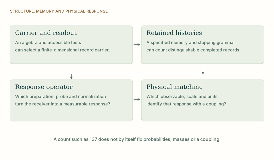
From carrier structure to a measurable response. Representation dimension, a chosen retention grammar, a response operator and physical calibration are separate stages of the constants programme. View full size ↗
03How Spin networks and spin foams frames the problem
Spin networks label quantum geometric states by representations and invariant intertwiners. Spin foams organize amplitudes for transitions between such boundary states. These structures are not automatically networks of ordinary matter particles, even when the same representation groups appear in particle physics. Constraints determine which labels encode geometric degrees of freedom.
DTT can use this comparison to clarify how local carriers are sewn into a global record. The crucial questions are which amplitudes the sewing rule assigns, which redundancies are removed, and what continuum observables emerge. A completed history resembles a boundary-to-boundary construction only after those maps have been defined; visual similarity between diagrams cannot establish equivalence. [4][5]
04Where the mechanisms agree and differ
Spin-network state counts and representation dimensions are exact combinatorial quantities, but they do not directly determine the electromagnetic fine-structure constant. Most spin-network labels concern quantum geometry, while an electromagnetic response requires a charged matter sector and a gauge action. DTT's retained-record count faces the same distinction between counting states and measuring an interaction.
A useful bridge would couple a physical carrier to a neutral reference and calculate the completed loop response. The relevant coefficient could then depend on representation dimension or on the rank of an invariant projector. Six nested inner levels might organize the sewing process, but they do not automatically choose the decimal weights in the 137 formula. The worked arithmetic below makes those weights explicit. A strong temporal construction would show why a specific count appears in an observable response, rather than simply in the dimension of an auxiliary space. It would also account for inaccessible sectors that cannot affect the experiment. This is particularly important because adding unobservable internal states can change a raw count while leaving all normalized amplitudes unchanged. The physical constant must be tied to what the carrier actually measures. [4][5]
05Worked example: assumptions, calculation and result
For d=0,1,2,3, compute 2ᵈ−1 to obtain 0,1,3,7. Then Σ(2ᵈ−1)10^(3−d)=0+100+30+7=137. The arithmetic is exact. Replacing the radix by a general b gives b²+3b+7, so b=9 gives 115 and b=11 gives 161. The choice of base therefore has physical importance if the result is intended as an invariant response rather than a notation.
Using the rounded measured inverse α⁻¹≈137.035999, the difference from 137 is about 0.035999. Relative to 137 this is approximately 2.63×10⁻⁴. This is the size of a matching correction, not its derivation. Calling it holonomy or mass dressing becomes explanatory only after an independently fixed model calculates its sign and magnitude. [1][2][3]
All quantities in this counting exercise are dimensionless. The measured inverse is rounded; the calculation does not equate a structural label with α⁻¹.
06An independent operational check
A response can be insensitive to an enlarged auxiliary space. If extra states never couple to the charged carrier and are traced out with unit normalization, multiplying their number need not change any scattering probability. Consequently, a raw dimension cannot determine α unless the completion dynamics makes that dimension enter a physical coefficient. This is a stringent but useful test of the retained-record proposal. It distinguishes an observable normalization from bookkeeping and asks whether the proposed 137 survives removal of inaccessible or redundant sectors. A count that passes this test would be a much stronger candidate for physical matching than an integer obtained from an unconstrained state catalogue.
07What follows from the comparison
The productive comparison is between response mechanisms. A structural theorem can reduce the available vacuum organization; field theory then tells us what matching and radiative corrections mean. A strong SMM/DTT result would fix the electromagnetic response in one declared scheme and derive an additional observable using the same inputs. That would turn an intriguing number into a constrained physical proposal.
THE SAME QUESTION, DIFFERENT STARTING POINTS
The comparison at a glance
Question
SMM/DTT
Spin networks and spin foams
Starting physical structure
One nonspatial source; six nested inner functional levels produce records accessible through outer completion.
Representation-labeled graphs, invariant intertwiners and transition amplitudes.
The central mechanism in this topic
Only record sectors that affect a physical charged response can contribute to coupling matching.
Representation dimensions and invariant network counts are geometric or algebraic data.
How the claim is made operational
A source-to-record map must define geometry, material response and physical clocks with shared inputs.
Gauge-invariant sewing, constraint implementation and semiclassical geometric amplitudes.
Meaning of agreement
Agreement is a compatibility result; a source-selected relation or fixed residual would add explanatory content.
The stated framework provides a benchmark within its own assumptions and established domain.
KEEP THE CONNECTION
Key ideas
A measurable loop response is a stronger target than the dimension of an auxiliary state space.
The worked example establishes only the result stated under its explicit assumptions.
Six nested inner levels describe one generative organization; outer time orders accessible completion.
Develops the source construction or operational distinction used in this comparison.
Sources and further reading
References support the comparator and the specific mathematical or interpretive claims indicated. SMM/DTT connections are developed in the analysis above.
NIST, CODATA value: fine-structure constant ↗Official metrology reference for the measured fine-structure constant; consulted 17 October 2026, values below are deliberately rounded.