Structural 128 and 137: from vacuum labels to measured couplings
Exact 128 and 137 can be meaningful structural labels without being measured running couplings. The decisive question is how a chosen vacuum sector affects a physical response. This guide preserves the intended SMM/DTT interpretation, gives an exact finite-state calculation, and shows why different observables can extract different coefficients from the same state count.
In the intended SMM/DTT programme, 128 and 137 describe distinct structural vacuum organizations associated with particular readouts. They should not be identified by numerical proximity with electromagnetic couplings at two energy scales. The physical electromagnetic response is defined through an action or a measurement and depends on normalization, matter content and matching.
DTT's six nested inner levels organize generation, while outer completion determines which distinctions are retained. A count of retained states can therefore be a real mathematical output. The next question is whether the count controls an observable response and why. This guide does not invent a missing derivation of the 128 sector; it treats the integer as a structural target whose physical map must be supplied by the actual source model. [1][2]
02Worked neutral-amplitude example
Take a D-dimensional carrier and a matching reference with normalized state |s⟩=D⁻¹/²Σa|a⟩|ā⟩. Apply a phase e^(iθ) to one carrier basis state and leave the others unchanged. The neutral return amplitude is A(θ)=⟨s|(Uθ⊗I)|s⟩=(D−1+e^(iθ))/D.
Its real part is 1−(1−cosθ)/D, so the curvature −d²ReA/dθ² at θ=0 is exactly 1/D. But the return probability is P(θ)=|A(θ)|²=1−2(D−1)(1−cosθ)/D², whose curvature is 2(D−1)/D². The same state count therefore yields different response coefficients depending on which observable is measured. A dimension alone does not choose the physical normalization.
D is a positive integer and θ a dimensionless applied phase. This is an explicit illustrative carrier/reference model, not an asserted derivation of a DTT vacuum sector.
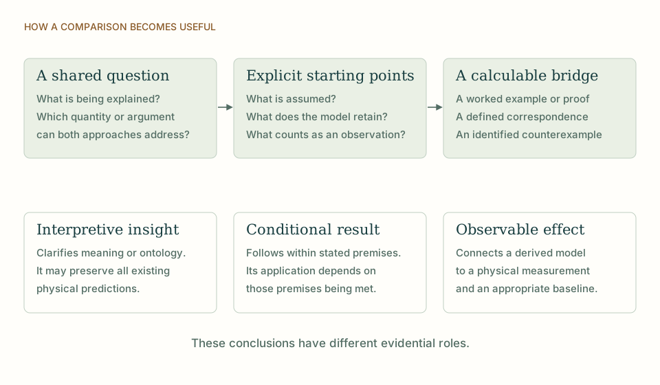
A comparison that reaches a definite conclusion. Begin with the same question, identify what each approach assumes, and compare a shared result. An interpretation, a conditional theorem and an observable deviation have different evidential roles. View full size ↗
03What the numbers show
For D=128, the amplitude curvature is 1/128≈0.0078125, while the probability curvature is 254/16384≈0.015503. For D=137, the corresponding values are approximately 0.007299 and 0.014492. Neither coefficient is automatically the electromagnetic fine-structure constant. The experiment and interaction determine which response, if either, has that meaning.
The example is useful because it supplies a positive mechanism: a normalized coherent neutral amplitude can produce an exact inverse dimension. It also exposes the required physical choices. The source must specify the carrier, reference, perturbation and readout, and show why the measured coupling is proportional to that particular curvature. A different phase applied to several basis states, a different reference state or a probability-based readout changes the coefficient.
04Canonical normalization is an additional calculation
Suppose a source response enters an effective gauge Lagrangian as −ZF²/4+qAμJμ in rationalized natural units. After Acan=√Z A, the measured charge is e=q/√Z and α=q²/(4πZ). To identify an inverse response count with α⁻¹, the model must derive the relation 4πZ/q²=C for the relevant structural value C.
This cannot be inferred solely from the neutral amplitude. The phase θ itself may contain q, and the conversion between a phase perturbation and a physical electromagnetic field carries units and normalization. Six nested inner levels could constrain those quantities, but the actual action-level calculation is indispensable. A source-selected coefficient that survives this matching would be a genuine coupling prediction.
α=q²/(4πZ); identifying α⁻¹ with C requires a derived 4πZ/q²=C.
Four-dimensional natural units; Z>0 and a specified current normalization are assumed.
05Why auxiliary states may be irrelevant
Suppose an extra sector is completely decoupled from the charged carrier and is traced out with unit normalization. Increasing its dimension changes the total Hilbert-space count but leaves all measured carrier probabilities unchanged. Therefore only states that enter the physical response with derived weights can contribute to a coupling formula.
A completion construction should identify redundant descriptions, inaccessible sectors and genuinely responding states separately. This is not merely a bookkeeping concern: it determines whether an integer survives changes of representation. A structural count has the strongest physical claim when the source rule makes it invariant and when removing an unobservable auxiliary factor does not alter the predicted coupling.
06Mass and holonomy dressing
The measured low-energy inverse electromagnetic coupling is approximately 137.035999. Its difference from the structural integer can be a target for a correction calculation, but calling the difference mass dressing or holonomy does not determine it. The source model must calculate the correction with parameters fixed independently and state the matching convention.
The 128 sector then needs its own observable interpretation. It may characterize a different completion response, a different vacuum organization or an internal structural relation. None of those meanings requires equating it to a high-energy running coupling. Preserving this distinction makes the programme stronger because the exact mathematical labels can remain exact while physical observables are obtained through a transparent, testable response map. [1][2]
07A comparison that could fail for a useful reason
The amplitude example predicts a definite relation between two responses measured on the same carrier. If the physical completion apparatus measures probability rather than coherent amplitude, the inverse-dimension coefficient is not the relevant result. Discovering this would not invalidate the state count; it would invalidate that particular coupling identification. This is a useful form of falsifiability within the model. The source programme becomes stronger when the readout instrument is fixed before its response is compared with a measured constant, because the calculation can then genuinely support or reject the proposed bridge.
08A concrete positive research target
The finite-state calculation identifies an attainable result: derive a physical neutral-amplitude response proportional to the inverse retained dimension, then prove that the same source fixes its conversion to a gauge kinetic coefficient and charge normalization. A second observable calculated from the same carrier would test whether the relation has real predictive content. That would connect 128 and 137 to physics through a mechanism rather than through numerical resemblance.
THE SAME QUESTION, DIFFERENT STARTING POINTS
The comparison at a glance
Question
SMM/DTT
Response normalization and effective coupling matching
Structural labels
128 and 137 denote specified vacuum/readout organizations in the intended programme.
Measured couplings require an operational definition and scale convention.
Response
A coherent amplitude can produce 1/D under explicit carrier/reference assumptions.
A probability curvature from the same model gives 2(D−1)/D² instead.
Physical matching
The source must derive the action and charge normalization connecting the count to α.
Canonical normalization and radiative matching determine the measured interaction.
KEEP THE CONNECTION
Key ideas
128 and 137 denote specified vacuum/readout organizations in the intended programme.
A coherent amplitude can produce 1/D under explicit carrier/reference assumptions.
The source must derive the action and charge normalization connecting the count to α.
Develops the source construction or operational distinction used in this comparison.
Sources and further reading
References support the comparator and the specific mathematical or interpretive claims indicated. SMM/DTT connections are developed in the analysis above.
NIST, CODATA value: fine-structure constant ↗Official metrology reference for the measured fine-structure constant; consulted 17 October 2026, values below are deliberately rounded.