Temporal generation and locality: what a Lieb–Robinson bound proves
A finite speed of influence is an important part of emergent spacetime, but a propagation bound assumes an interaction structure. DTT asks the additional question of how that structure is generated. This article separates neighborhood preparation from transport, works through a bound, and identifies a joint result that would make temporal locality physically stronger.
Causal order and spatial proximity encode different information. A causal relation states which events can influence which others. A spatial distance compares records on an appropriate common slice or through a relational protocol. A graph can have a finite propagation speed relative to its edges while still being physically nonlocal if those edges join arbitrarily distant readouts.
Locality therefore has two stages: the interaction structure must be generated, and the dynamics must respect that structure. An inequality bounding propagation on an already chosen graph addresses the second stage. It does not explain why that graph resembles three-dimensional space. This separation makes the challenge sharper and gives partial achievements a clear place in the overall reconstruction. [1][2]
02The mathematical bound and its domain
For a quantum lattice or metric interaction system with suitably bounded, decaying interactions, a Lieb–Robinson inequality controls the commutator of observables supported far apart. Its characteristic form is ‖[A(t),B]‖≤C exp[−μ(d−vLR|t|)]. The constants depend on the interaction assumptions and observables. The inequality describes an effective cone with exponentially small tails; it is not in general an exact relativistic microcausality statement.
The important logical point is that d is already a metric or distance on the interaction structure. The theorem bounds influence relative to that supplied structure. It does not prove that the structure was generated from a nonspatial source, that its large-scale dimension is three, or that its effective speed equals the measured light speed. Those are independent questions to which DTT can contribute. [1]
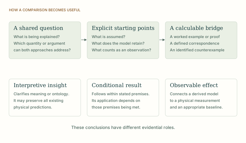
A comparison that reaches a definite conclusion. Begin with the same question, identify what each approach assumes, and compare a shared result. An interpretation, a conditional theorem and an observable deviation have different evidential roles. View full size ↗
03The source-based interpretation
The Single Monad is nonspatial, so its alleged unity cannot be represented as a point that sends ordinary signals from a hidden location. In DTT, locality would belong to the relations among completed records. The six inner levels could produce and retain a neighborhood structure; outer time would order observable influence through that structure.
A single controller is not enough to explain locality if it is allowed to update any record pair independently. A stronger rule lets the same retained relations restrict both record formation and later transport. Then memory is physically important: it preserves which comparisons count as nearby, rather than being an inert log appended after spatial interactions have already been assumed.
04Worked comparison: exact circuit cone and Hamiltonian tail
On a chain with nearest-neighbor updates, suppose a disturbance can cross at most one edge of length a during each completed interval δτ. A record N edges away cannot respond before Nδτ, giving an exact circuit cone with v=a/δτ. This uses a bounded-depth update with strictly local gates.
Continuous-time Hamiltonians generally give a different result: a Lieb–Robinson estimate bounds a distant commutator by a constant times exp[−μ(d−vt)]. The tail is small rather than exactly zero outside the effective cone. If d−vt=10/μ, the exponential factor is about 4.54×10⁻⁵. Neither result determines a physical speed until the edge length and the clock interval are independently identified. Nor does either prove that the source generated the chain. [1][2]
Tₘᵢₙ=Nδτ; d=Na; v=a/δτ. A Hamiltonian bound has the form ‖[A(t),B]‖≤C e^(−μ(d−vt)).
d and a are physical distances only after readout calibration; μ has inverse-distance units. C depends on observables and interaction assumptions.
05Why the same graph can tell two different stories
Imagine records whose displayed coordinates lie in a cube, but whose interaction graph includes an edge from one corner to the opposite corner. A local graph update can use that edge in one step. The propagation bound remains true in graph distance, while the displayed Euclidean distance suggests an apparent shortcut. Thus a proof of bounded graph propagation does not establish physical locality unless the graph metric and the readout metric are compatible.
A source model can address this by generating both the coordinate readout and the retained adjacency through the same rule. The rule must also prevent later inner operations from introducing arbitrary long links. The six nested levels could implement compatible local comparisons, but a global controller with unrestricted access would leave the selection unexplained.
There is also a preparation issue. If local graphs form only after conditioning on an extremely rare completion outcome, the success probability and resource cost are part of the physical result. An efficient autonomous preparation law would be a substantial advance. It would explain why observers inhabit a local sector, rather than merely proving that such a sector exists in a large state space. [1]
06A precise positive conclusion
The strongest attainable theorem combines three statements: completed records define a stable neighborhood structure; source interactions respect that structure; and independently measured clock and distance scales turn the resulting influence bound into a physical cone. The first two explain locality, while the third calibrates it. A shared limiting speed across matter species is a further universality result. This sequence preserves partial achievements and makes clear why one successful bound does not yet prove all of relativistic spacetime.
07How this connects to the wider programme
The same retained memory that makes neighboring records persistent can also support transport, gauge comparison and material clocks. That is where SMM/DTT has a distinctive unifying aim. A model that derives these functions jointly would remove independent choices. The comparison with Lieb–Robinson theory therefore strengthens the programme by identifying exactly which assumptions can be imported as mathematical tools and which source-selection claims still need their own proof.
THE SAME QUESTION, DIFFERENT STARTING POINTS
The comparison at a glance
Question
SMM/DTT
Lieb–Robinson bounds
Distance
Readout distance and interaction distance must be generated and compared.
A metric interaction structure is an assumption of the bound.
Propagation
The source must preserve neighborhoods during further completion.
The bound controls commutators under specified local interactions.
Physical speed
Clock and length calibration must come from independent source observables.
The bound supplies a model-dependent effective velocity parameter.
KEEP THE CONNECTION
Key ideas
Readout distance and interaction distance must be generated and compared.
The source must preserve neighborhoods during further completion.
Clock and length calibration must come from independent source observables.
Develops the source construction or operational distinction used in this comparison.
Sources and further reading
References support the comparator and the specific mathematical or interpretive claims indicated. SMM/DTT connections are developed in the analysis above.