Re-creation of space and Regge calculus

01Curvature from gluing

A curved geometry can be approximated by flat simplices joined along their faces. Curvature is then concentrated at lower-dimensional hinges, where the angles around a hinge fail to sum to the flat value. Regge's construction gives a way to write gravitational dynamics directly in terms of edge lengths and deficit angles.

This is attractive for DTT because geometry can be described by relational gluing data rather than by a pre-existing coordinate chart. The source programme, however, asks an additional question: why do particular records and gluing relations arise? Regge calculus specifies geometric data and varies an action; it does not by itself generate those data from one metaphysical source. The six nested inner levels could organize production and consistency of the gluing, but their existence does not choose edge lengths or an action. ^[1]

02Worked two-dimensional deficit angle

At a vertex of a flat equilateral triangulation, six triangles contribute angles of π/3 each, so the total is 2π and the deficit is zero. With five such triangles, the total is 5π/3 and the deficit is π/3. The geometry has positive concentrated curvature at that vertex.

A tetrahedral surface has four vertices, each meeting three equilateral triangles. Each deficit is 2π−π=π, so the total deficit is 4π. This agrees with the integrated curvature relation for a sphere-like closed surface, whose Euler characteristic is two. The calculation demonstrates how curvature can be encoded in discrete relational data. It does not determine the physical size of the triangles or the dynamics that selects the tetrahedron. ^[1]

03The DTT bridge: generating compatible local records

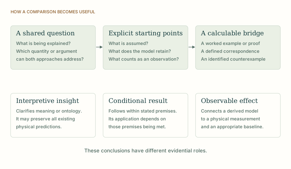
In a source-based construction, a completed local record could specify lengths, orientations or transport relations. Neighboring records must agree on shared data if they are to define one geometry. This gives the nested inner levels a concrete possible role: they can perform compatible local comparisons before a global outer record is retained.

A single controller is insufficient if it assigns each local patch independently and then forces consistency through an unrestricted global correction. The physical mechanism should explain how consistency is propagated and what resources it uses. If the source supplies an autonomous local rule that produces compatible simplicial data, Regge calculus offers a natural interface for assessing the resulting curvature. The construction would then be more than a picture of repeated spatial creation; it would generate a measurable geometry.

04From geometry to dynamics

In four-dimensional Regge gravity, a gravitational action involves a sum of hinge areas multiplied by deficit angles, together with the relevant normalization and boundary terms. The discrete action approximates the curvature integral in a suitable regime. A DTT source would need to explain why its history amplitudes or effective energy select this weight rather than an arbitrary function of the same geometry.

This is the same distinction encountered in continuum reconstruction: defining a metric or a deficit angle is kinematics, while selecting an action is dynamics. Six nested inner levels can organize both, but the source law must establish their relation. A successful result could be restricted to a semiclassical sector and still be valuable if it derives the action coefficient and identifies controlled corrections. ^{[1] [2]}

05Continuum matching of the action coefficient

Use natural units c=ħ=1 and consider S=∫d⁴x√−g[(M²/2)R−ρΛ+Lₘ]. With the usual definition Tₐᵦ=−2(δSₘ/δgᵃᵇ)/√−g and suitable boundary terms, variation gives M²Gₐᵦ+ρΛgₐᵦ=Tₐᵦ. Thus M²=1/(8πG) and Λ=ρΛ/M² reproduce the conventional Einstein equation.

The Bianchi identity ∇ᵃGₐᵦ=0 implies ∇ᵃTₐᵦ=0 when M and ρΛ are constant. If a proposed temporal rate makes M position dependent, derivatives of M enter the variation and the simple equation is no longer correct. This small calculation makes a useful diagnostic: a varying generative parameter cannot simply be inserted into a constant-coupling equation without accounting for its dynamics and energy exchange. ^{[2] [3] [4]}

06Re-creation versus re-triangulation

Changing a triangulation can be a change of regulator or description of the same physical geometry. Re-creation in DTT is intended as a physical production process. These meanings should not be conflated. A source model needs an observable clock and a history law before a sequence of triangulations represents physical evolution. Otherwise the sequence could simply be an algorithm for representing a static shape.

The comparison is strongest when the source generates compatible geometry and a physical update, while Regge methods provide independent curvature and dynamical checks. This would connect temporal generation to a well-defined discrete gravitational formalism without claiming that the formalism itself proves the source ontology.

THE SAME QUESTION, DIFFERENT STARTING POINTS

The comparison at a glance

Continue on SMONAD

• Generating a neighborhood and preserving local transport →

  Develops the source construction or operational distinction used in this comparison.

• Relational transport and gauge freedom →

  Develops the source construction or operational distinction used in this comparison.

• Noncommutative dual-time geometry: algebra, variation, distance →

  Develops the source construction or operational distinction used in this comparison.