
The scale factor organizes homogeneous distance changes. Standard conservation and gravitational equations determine its evolution; an SMM/DTT construction must generate the metric, clock, and source stress entering those equations.
Define the scale factor operationally
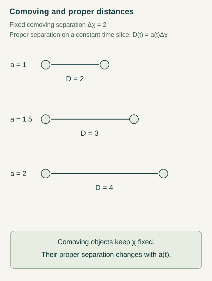
In a spatially flat homogeneous model, write ds²=−c²dt²+a(t)²d x². The coordinate x labels ideal comoving markers and has length units here; a is dimensionless and normalized to one at a chosen reference epoch. Two fixed markers separated by Δx have simultaneous proper separation d(t)=a(t)|Δx|.
Differentiation gives ḋ=Hd, where H=ȧ/a. The same fractional expansion applies to every pair of ideal markers. It does not imply that atoms or other bound systems expand with this law: their local forces and states must be treated separately from the homogeneous background.
Open the full-size diagram →
Derive the photon wavelength comparison
For a radial light ray in this metric, ds²=0 gives |dx|=c dt/a(t). Compare two closely separated wave crests emitted and received by comoving observers. They cover the same comoving path, so the small emission and reception intervals satisfy Δto/a(to)=Δte/a(te). Frequencies are inversely proportional to these intervals.
If the scale factor doubles during travel, the received wavelength doubles. This derivation assumes metric null propagation and comoving endpoints; peculiar motion and gravitational differences add further contributions in a more detailed observation model.
Energy dilution follows a fluid law
Let ε be energy density and p pressure, both in energy-per-volume units. For a separately conserved homogeneous perfect fluid, local conservation gives ε̇+3H(ε+p)=0. It can also be read as d(εV)=−p dV for a comoving volume V proportional to a³. Assuming constant equation-of-state ratio w=p/ε allows direct integration.
Pressureless matter has w=0 and scales as a−3. Radiation has w=1/3 and scales as a−4. A separately conserved constant vacuum contribution has w=−1. Exchange between sectors modifies their separate equations while preserving the total balance.
Worked example: doubling the scale
Normalize a=1 initially and double it to a=2. The proper volume of a fixed comoving cell grows by eight. Conserved nonrelativistic particle number therefore gives one eighth of the initial matter density. Radiation loses the same number-density factor and an additional factor two from photon redshift, giving one sixteenth of its initial energy density.
A constant vacuum energy density remains unchanged in this comparison, so its energy within the enlarged cell increases eightfold. The negative pressure accounts for this behavior in the local conservation equation. It should not be interpreted as a statement that an expanding universe possesses a single globally conserved Newtonian total energy.
Geometry needs an evolution equation
For the flat metric, Einstein gravity with constant G and a separately written cosmological constant gives H²=8πGε/(3c²)+Λc²/3 and ä/a=−4πG(ε+3p)/(3c²)+Λc²/3. Here ε and p exclude the vacuum contribution already represented by Λ, avoiding double counting.
For one conserved component with w>−1 and Λ=0, the expanding solution is a proportional to t2/[3(1+w)] after choosing the origin of time. Pressureless matter gives t2/3 and radiation t1/2. These follow by inserting the dilution law into the first equation and integrating; they are not independently chosen expansion schedules.
Distinguish expansion from finer resolution
A source may create more record distinctions while representing the same physical region more finely. That is refinement, not necessarily expansion. For example, dividing every cube into eight children doubles spatial resolution while leaving its total physical volume unchanged. Counting new cells alone cannot determine whether the world has grown.
An SMM/DTT expansion variable should therefore compare persistent comoving markers using independently calibrated distances. Their mean separation could change because the effective metric changes, while the detector resolution evolves in another way. The same distinction applies to a growing archive: additional records do not automatically imply additional spatial volume.
The rate must use a material clock
If a source label s orders completed configurations and the physical clock satisfies dt=N(s)ds, the measured expansion rate is H=(1/a)(da/ds)/N(s). The scale sequence alone does not fix H. Choosing a different clock coupling can change inferred dynamics while preserving exactly the same ordered geometries.
The six inner stages must generate dependent formation work and clock-compatible completion, rather than serve as six independent adjustable expansion parameters. A source law that fixes both the distance change and the clock lapse would make the cosmological rate a joint prediction.
What a temporal cosmology should recover
A first constructive result could derive an approximately homogeneous metric and an effective conserved stress tensor, then recover the simple matter and radiation solutions in their appropriate regimes. It should specify why local bound structures remain stable, how photons acquire redshift, and which approximation produces the macroscopic clock.
A more ambitious result would constrain a correction shared by expansion and structure growth. Adding an arbitrary function to H(t) can fit many histories, but it does not explain their origin. The useful SMM/DTT contribution is a relation forced by one update and retained across independently defined observables.
Continue with the articles
- Summary of Modern Theories of Cosmology
Map the conceptual transition toward modern cosmology, highlighting the roles of gravitation, observation, and cosmic evolution. Explain where SMM proposes a different starting point.
- The Principle of Ever-renewed Creation
Introduce ever-renewed creation as a central motivation of the Single Monad Model. Ask how the idea might be expressed through histories, completed records, and observable persistence.
- From record refinement to a joint clock–band relation
Introduce the conditional relation connecting geometry, clock response, and matter transport. Explain why the interfaces and coefficients must be independently calibrated.
- A finite-update cone
Introduce the bound relating horizontal displacement to temporal projection in the limiting-speed draft. Explain that the finite-update inequality is a stated geometric assumption.
- Counting records to recover volume
Explore the archive and sampling assumptions used to connect normalized record counts with homogeneous four-volume. Compare a Poisson benchmark with the separately specified autonomous sampler.