
A four-position hopping model with a supplied singlet penalty reduces to one strictly monotone resolvent equation. Its finite auxiliary gap is protected, while its physical origin and continuum interpretation remain separate questions.
Supply a mobile carrier and a stationary reference
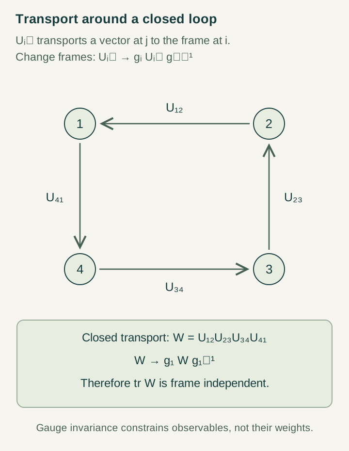
Take four positions arranged on a loop. At each position the mobile object has an m-dimensional complex internal carrier. A stationary dual of the same dimension remains at the root. The full auxiliary space has dimension 4m². At the root, define the normalized singlet s=m−1/2Σa|0,a⟩|ā⟩.
The reference makes the neutral contraction independent of a basis choice. SMM/DTT can interpret a completed loop as a comparison between mobile generative work and a retained reference. The mathematics begins with the graph, carriers, link maps, and their physical availability already supplied. The interpretation becomes a source construction only if those ingredients are generated by an explicit update.
Open the full-size diagram →
A positive singlet penalty and coherent hopping
Let K be the Hermitian hopping operator with real amplitude t and unitary links around the four edges. Choose a penalty Δ>0 and set H=Δ(I−|s⟩⟨s|)−K. The penalty makes the root singlet the zero-energy state before hopping is introduced; every orthogonal state initially costs Δ.
The penalty is a physical input, not a consequence of frame invariance. Gauge covariance determines how links and carriers transform, but many different invariant Hamiltonians are possible. This model is valuable because it isolates one such choice and permits an exact response calculation without a small-hopping approximation.
Preparing the root singlet is also distinct from preparing the interacting ground state. Once hopping is active, the ground vector spreads over the loop. An experiment measuring its static energy must specify how that state is prepared or how its eigenvalue is inferred from a controlled response.
Reduce the links to their total holonomy
Changes of local frame can set three links to identity, leaving the complete holonomy W on the remaining link. Diagonalize W with eigenvalues exp(iθa). In each internal channel the mobile problem becomes a four-site ring with a twisted boundary condition.
The displayed free eigenvalues determine the singlet resolvent, with weight 1/(4m) for each channel and ring mode. Degenerate eigenvalues combine their weights. This reduction shows why the static response depends on closed-loop transport rather than on arbitrary individual link matrices.
One equation selects the ground energy
Write the lowest energy as E₀=Δ−z. The rank-one perturbation equation gives:
z>λ*=maxa,kλak.
Above the free spectral edge, every denominator is positive. The resolvent is strictly decreasing, diverges at the edge, and tends to zero at infinity. It crosses 1/Δ exactly once, yielding a unique ground state. The branch inequality is essential; multiplying denominators into a polynomial can create additional roots that do not describe this state.
At t=0 all free eigenvalues vanish, R=1/z, z=Δ, and E₀=0. This simple limit checks the normalization and energy convention.
A finite gap with an explicit lower bound
Let w* be the singlet weight in the highest free eigenspace. The top term of the resolvent gives 1=ΔR(z)≥Δw*/(z−λ*), hence z−λ*≥Δw*. Rank-one eigenvalue interlacing bounds the next perturbed level by the old spectral edge.
For m=2 the bound is Δ/8; for m=3 it is Δ/12. At zero hopping the actual gap is Δ, illustrating that the uniform estimate is not an equality at every parameter value. The theorem protects this finite auxiliary spectrum. It does not address an infinite-volume gauge-field Hilbert space or removal of a continuum regulator.
Energy and a one-shot return probability differ
The ground energy is determined by the full resolvent and, in this supplied static model, is minimized at identity holonomy. A different protocol prepares s, applies W only to the mobile factor, and tests neutral return. Its probability is |tr W|²/m².
These observables contain different information. For a central phase W=exp(iθ)I, the return probability is one for every θ, while the static twisted-ring energy generally changes with θ. The probability discards a common return phase; the hopping dynamics compares it through alternative excursions. A temporal completion interpretation must identify which experiment is meant before using one quantity as a proxy for the other.
What the exact model contributes to SMM/DTT
The construction supplies a finite, fully normalized target: a unique ground response, a measurable loop dependence, and an auxiliary gap that survives arbitrary permitted holonomy. It can support controlled elimination when additional scale conditions make a perturbative expansion accurate. Gap protection and approximation accuracy are different tests.
The next source-level task is to realize the stationary dual, the neutral penalty, and the unitary links from the nested generative operations. A successful derivation should calculate Δ and t relative to independent physical standards, specify how completion is registered, and retain errors under coupling to other records. That would convert an exact model contribution into a selected physical mechanism.
Continue with the articles
- An exact singlet-loop response
Introduce the four-position mobile carrier and stationary dual used in the solvable model. Explain how the holonomy-dependent resolvent determines the ground-state response under the supplied Hamiltonian.
- A protected gap in the finite singlet model
Explain the model’s unique ground state and gap bound. Distinguish a finite-system spectral statement from a continuum mass gap in a physical gauge theory.
- What the holonomy Hessian does and does not contain
Explore the exact trace structure of the response near identity holonomy. Explain why the absence of an independent squared-trace term matters for the model’s coefficient relations.
- Controlled effective gauge Hamiltonians
Introduce the finite-cell effective Hamiltonian and its explicit remainder. Explain why a controlled approximation needs a stated norm bound and an evolution-error estimate.