
For a direct sum of normalized two-site edge blocks, the commutator bound is exactly an edge-slope bound. Maximizing admissible record differences then reproduces weighted shortest-path distance, including its calibration and stability properties.
What a distance measurement compares
Suppose completed records are vertices of a connected graph and each edge e has a positive calibrated length ℓe. A real observable f assigns a reading to every vertex. Calling f one-Lipschitz means that its reading changes by at most ℓe across each elementary comparison.
The distance between two records can then be recovered as the largest possible difference of readings among all such observables. This operational viewpoint fits SMM/DTT: source operations create relations, completion makes them available, and comparison tests determine their geometric meaning. The following construction makes the relation between local tests and global distance exact.
A normalized two-site block
For an edge joining x and y, represent f by the diagonal matrix with entries f(x),f(y). Use an off-diagonal comparison operator with entries 1/ℓe. Taking a direct sum of these blocks over all edges keeps their normalizations separate.
L(f)=‖[D,f]‖=maxe={x,y} |f(x)−f(y)|/ℓe.
The commutator has off-diagonal entries proportional to f(y)−f(x), so its norm is the absolute edge slope. The norm of a direct sum is the maximum block norm. This exact equality depends on the chosen block construction; a generic adjacency matrix need not reproduce it.
Why the global distance is the shortest path
If L(f)≤1, the reading difference across every edge is bounded by its length. Sum along any path from x to y. The triangle inequality bounds |f(x)−f(y)| by that path's total length, so the supremum over admitted f cannot exceed the shortest-path distance.
For the reverse inequality, choose f(z)=distG(z,y). Moving across one edge changes this distance by at most that edge length, making f admissible. Its difference between x and y equals their shortest-path distance. The upper bound is therefore attained.
Worked example: three records and three comparisons
Let A–B have length two, B–C length three and A–C length seven. The direct comparison allows a difference of seven, but the two-edge route imposes a tighter total limit of five. Hence the actual distance from A to C is five.
Edge slopes: 1, 1, 5/7; therefore L(f)=1.
This f attains the distance. If the direct edge is shortened to four, the distance becomes four and f=(0,2,4) is admissible. Local comparisons therefore constrain one another globally; the metric is not obtained by reading the largest single edge label.
Open the full-size diagram →
A cubic graph does not automatically give Euclidean distance
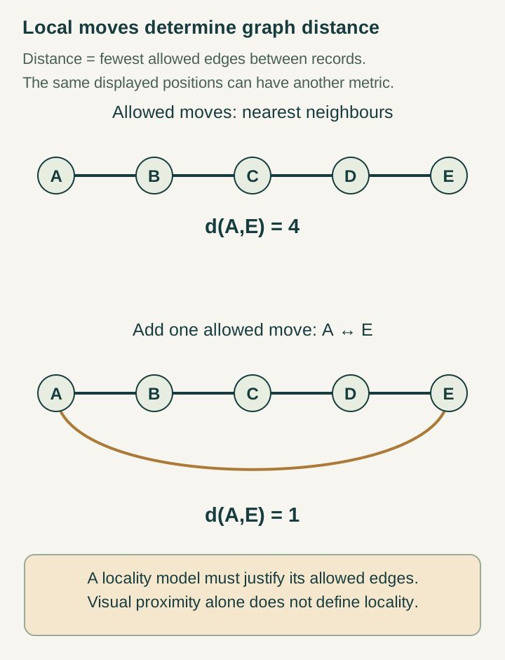
On a cubic lattice with unit axial edges, graph distance between integer coordinates is the sum of absolute coordinate differences. Between (0,0,0) and (1,1,0), this is two. The Euclidean straight-line distance in an embedding is √2. Both are coherent metrics, but they describe different comparison procedures.
Refining axial edges while retaining their unit path-cost rule preserves this Manhattan norm at large scales. An isotropic Euclidean limit needs additional probe directions, suitable averaging or another explicitly derived comparison law. Cubic volume growth identifies a dimension; it does not select which norm measures length. The source must explain the actual observer's comparison operations.
Counting modes is a different diagnostic
A frequency operator can have eigenvalue count proportional to a cutoff cubed and still fail to compare record locations. If both the operator and all allowed observables are diagonal in the same basis, every commutator vanishes. Arbitrarily large differences between distinct evaluation states then satisfy L(f)=0, giving infinite spectral distance.
The missing ingredient is a coupling that compares records, such as the edge blocks above. Spectral dimension, metric distance and propagation consequently require separate tests. The three can agree in a successful model, but their agreement is informative precisely because one does not follow automatically from the other.
Scale and error bounds
Multiplying every edge length by a positive factor a divides D by a and multiplies every distance by a. The graph and dimension are unchanged. A physical ruler therefore needs an independently fixed normalization, tied to the completion or material processes used to implement comparisons.
There is also a useful stability result. Suppose each perturbed edge length lies between (1−ε)ℓe and (1+ε)ℓe, with 0≤ε<1. Every path length satisfies the same two-sided bound. Minimizing over paths gives:
What the source must generate next
The comparison construction provides a concrete task for SMM/DTT: generate persistent links, positive edge calibration and connected access through one declared source process. If the graph is disconnected, functions constant on each component can differ arbitrarily between components while retaining zero slope. Distances across those components are infinite.
A promising extension would derive edge weights from an observable response of completed records and compare that response with material clock readings. It should also test whether refinement preserves distances between fixed physical landmarks. This would connect the exact finite metric to the larger goal of a common origin for geometry, duration and matter.
Continue with the articles
- Programmed geometry and spontaneous selection
Compare the draft’s explicit torus preparation with a mechanism that would naturally select geometry. A constructive example proves feasibility while leaving the physical origin of its program open.
- A spectral triple as a reconstruction interface
Introduce the algebra, Hilbert space, and Dirac-type operator used by the temporal spectral model. Explain the different jobs of observables, states, and spectral data.
- Three-frequency counting and inner spectral dimension
Introduce the cubic eigenvalue-counting result for the inner operator. Explain why including the separate outer circle changes the count in the compact auxiliary model.
- Why spectral dimension does not determine distance
Use the draft’s counterexample to show that an operator can have a useful eigenvalue count while giving infinite distances between localized states. Dimension and metric require separate checks.
- Graph distance from a normalized spectral block
Introduce the graph-block construction whose Connes distance equals weighted shortest-path distance. Explain the normalization assumptions behind that equality.
- A finite regulator for spectral experiments
Outline a reproducible finite-model exercise comparing eigenvalue counts, heat traces, and graph distances. Use it to show which diagnostics converge together and which measure different features.