
Present readability and predictive completeness are different requirements. For a finite linear update M and retained projection P, autonomous prediction is possible exactly when PM(I−P)=0; otherwise additional state or explicit memory is needed.
1. One source is a starting commitment
The Single Monad Model (SMM) proposes a common generative source for the many relations that observers describe as a world. Duality of Time Theory (DTT) develops a distinction between generative activity and completed observable order. These ideas become mathematical when the source has a declared state, an update law, a preparation rule, and a way to export records. The word “one” does not supply those objects automatically. A single computer can execute many incompatible programs; likewise, a single carrier can support many inequivalent dynamics.
This chapter makes one part of the programme precise: what information must a completed record retain if it is to support future predictions? The answer depends on the allowed experiments. Two source states can look identical now and become distinguishable after an admitted operation. An adequate predictive record must preserve that distinction, or represent its effects through memory.
We use deterministic finite systems first, then a linear differential example. Their assumptions are visible: a state space X; composable operations h; a completion map Q; and tests o on completed outputs. Probability, Hilbert space, spatial locality, and physical clock calibration are not consequences of that list. They can be added, but each adds mathematical content. Keeping this first layer small makes it possible to identify exactly which conclusion has been established.
In the six nested inner roles described elsewhere on this site, successive stages organize dependencies within generation before export. Here a completed operation can represent the whole nested cycle. It need not be a single elementary step, and the number of internal roles is not inferred from the number of variables in an example.
2. Define equality by completed future tests
Let Hist be a monoid: operations can be composed associatively, with an identity operation e. Fix a convention in which hk means “apply k, then h.” Its action satisfies (hk)·x=h·(k·x). Let Q:X→Comp map the source state to a completed record. A set O of tests specifies which properties of that record can be read. Define an equivalence relation by requiring all admitted future experiments to agree:
for every admitted future history h and test o.
Reflexivity and symmetry follow from equality; transitivity follows by comparing each fixed pair (h,o). More importantly, this is the coarsest relation preserving the declared experiments. If another relation R identifies only states giving equal results in every such experiment, then R is contained in ≡. Thus the quotient retains precisely the distinctions the test family can expose.
To obtain an update on equivalence classes, the future histories must be closed under the appropriate composition. If x≡y and a is an allowed update, every test following a is a test of ha. Closure gives h·(a·x) and h·(a·y) equal completed outcomes, so a·x≡a·y. Without that closure, a list of tests can define an equivalence relation without defining autonomous quotient dynamics.
The choice of tests is substantive. Enlarging the family can split old classes into smaller ones. A detector that reads only a bit can have a smaller present display than the predictive state required when controlled future transformations are also allowed.
3. Worked example: the missing sign
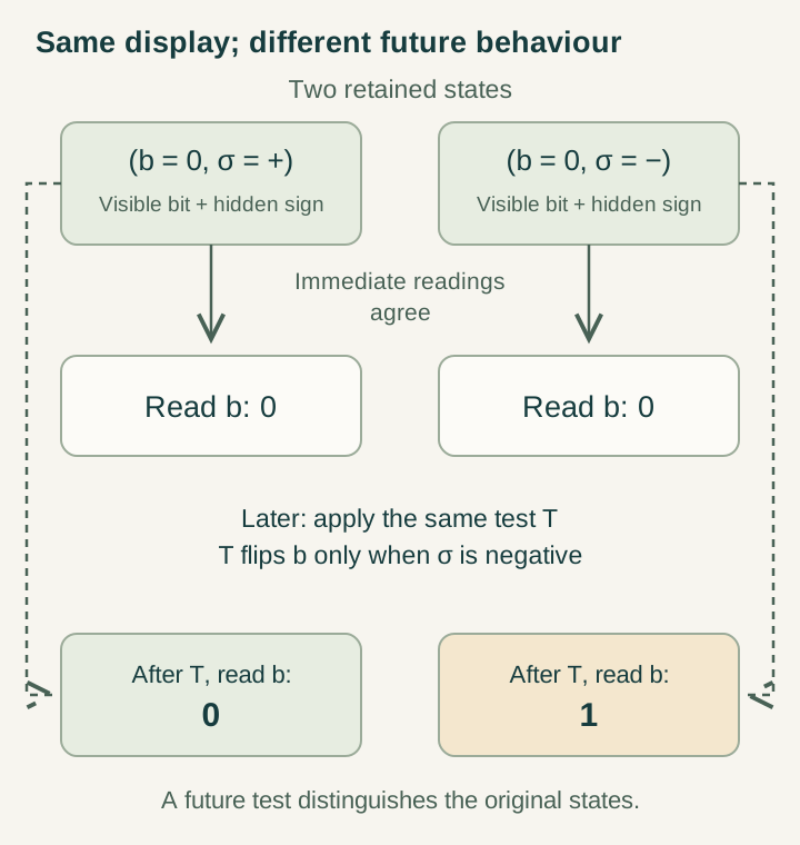
Take four source states (b,σ), with b∈{0,1} and σ∈{+1,−1}. The immediate observation is ρ(b,σ)=b. Define T to flip the bit exactly when σ=−1, leaving the sign unchanged. Then ρ(0,+1)=ρ(0,−1)=0, but ρ(T(0,+1))=0 and ρ(T(0,−1))=1. No map on the displayed bit alone can reproduce both next observations.
If the allowed tests consist only of “read now,” there are two observable classes. If they include “apply T, then read,” all four states are distinguishable: the first reading determines b and the second reveals whether it flipped. The extra predictive information is one bit. It is not an extra spatial dimension or evidence for a second physical clock.
A probabilistic state can retain less specific information when the preparation is uncertain. Write p for the conditional probability that σ=−1. The chance of a flip is p; after observing a result, update the conditional distribution. Such a distribution is an additional statistical construction, not a consequence of merely naming the hidden sign. In a physical model its preparation and measurement rules must be specified.
The example clarifies a useful meaning of completion: a record may be complete for a declared experiment while remaining incomplete for a richer one. SMM/DTT can therefore distinguish completion of an output from erasure of every internal distinction. A claim of complete predictive closure must say which future operations are included.
4. Derive the finite linear closure test
Let z be a vector in a finite-dimensional real inner-product space, with one-step update z′=Mz. Let P be an orthogonal projection onto retained coordinates, and write r=Pz and h=(I−P)z. Projecting the update gives r′=PMP r+PM(I−P)h. We seek a single linear map B on retained states such that PMz=BPz for every full state z.
When it exists, B=PMP restricted to ran P.
Necessity follows by taking z in ker P: its retained value is zero, so any autonomous linear update must return zero. Sufficiency follows by inserting the decomposition z=Pz+(I−P)z. The criterion is exact and makes no assumption that M is unitary, reversible, or dissipative.
For example, choose M with rows (1,1) and (0,1), and retain only the first coordinate. States (0,0) and (0,1) have the same present output but next outputs zero and one. The neglected component leaks into the display. If the omitted state has norm at most ε, the one-step prediction error made by ignoring it is bounded by ‖PM(I−P)‖ε. A small leak is an approximation with an error scale; a zero leak is an exact autonomous quotient.
Closure can also occur only at a chosen completion interval. A quarter-turn rotation of a plane exchanges the retained and hidden axes, so a one-step display is not autonomous. Four turns multiply to the identity, which is autonomous on every projection. This construction explains why the product of a cycle must be tested, rather than assigning closure to every unfinished inner stage.
5. Compute how much predictive memory is needed
For a linear readout y=Cz and update M, all future observations are C Mⁿz for n≥0. The invisible subspace is N=⋂ₙ≥₀ ker(CMⁿ). Two states are predictively equivalent exactly when their difference belongs to N. Because M maps N into N, it induces a well-defined linear update on the quotient by N.
In a d-dimensional system, the Cayley–Hamilton theorem expresses Mᵈ as a combination of lower powers. Hence it is enough to intersect the first d kernels, or equivalently compute the rank of the stacked observability matrix with rows C, CM, …, CMᵈ⁻¹. That rank is the dimension of the minimal deterministic linear predictive quotient for this readout. It need not equal the number of displayed components.
y₀=z₁+z₂, y₁=z₁+2z₂
z₂=y₁−y₀, z₁=2y₀−y₁.
The display is one-dimensional, yet two successive values distinguish the full two-dimensional state. The output obeys yₙ₊₂=3yₙ₊₁−2yₙ, so two retained readings suffice for a local recurrence. Recording only the latest value does not. This is a concrete alternative to treating all hidden information as permanently unknowable.
For SMM/DTT, the test suggests a constructive research procedure: specify the completed readout and source update, calculate the invisible subspace, and compare the resulting predictive memory with the proposed record grammar. A dimensional count should describe a declared task, rather than change meaning between present observation, future prediction, and internal storage.
6. Eliminate a hidden mode without losing its influence
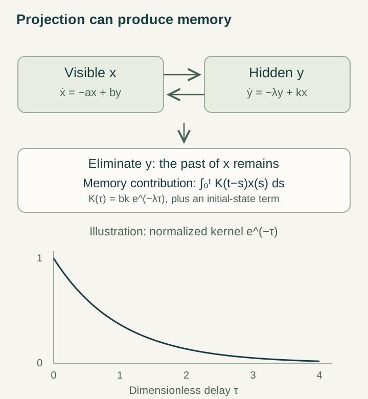
Now let an observed variable x and hidden variable y obey ẋ=−ax+by and ẏ=−λy+kx, with λ>0. Multiplying the second equation by exp(λt) makes its left-hand side a total derivative. Integrating from the preparation time zero gives y(t)=exp(−λt)y(0)+k∫₀ᵗexp[−λ(t−s)]x(s)ds. Substituting this expression into the first equation produces:
+∫₀ᵗK(t−s)x(s)ds, K(τ)=bk exp(−λτ).
There are two retained influences. The initial hidden preparation supplies an inhomogeneous term; subsequent observed history supplies the convolution. Dropping either changes the problem unless the preparation or approximation justifies it. The system is local in the pair (x,y), but generally history-dependent in x alone.
With zero initial hidden state, the Laplace-domain kernel is K̂(s)=bk/(s+λ). A finite sum of exponential kernels can likewise be represented with finitely many auxiliary modes. This identifies a precise comparison class: such memory may admit an ordinary one-parameter state-space realization. Observing it does not, on its own, distinguish one-time from dual-time ontology.
7. Memory is distinct from relaxation and a temporal arrow
The full matrix of this example has trace −(a+λ) and determinant aλ−bk. For real coefficients, both eigenvalues have negative real parts exactly when a+λ>0 and aλ−bk>0. With a=2, λ=3 and b=k=1, its characteristic polynomial is s²+5s+5; both roots (−5±√5)/2 are negative. Increasing b to seven makes the determinant −1, so one mode grows. The memory kernel still decays as a function of its delay.
Thus a decaying kernel does not guarantee a decaying solution. Nor does a stable matrix identify physical entropy. A stable finite matrix admits positive quadratic Lyapunov functions, but calling one of them thermodynamic free energy requires an independently justified energy and bath interpretation.
Reversible full dynamics also requires care. If an entire invertible group action descends through the same quotient, its descended inverse remains an inverse. Irreversible record dynamics can instead arise when only a future semigroup is admitted or when preparation and discarding remove accessible inverse information. A two-sided sequence shifted reversibly becomes a one-sided future sequence under a tail readout; the forward tail shift loses its first bit and has no unique inverse.
The distinction matters for DTT: ordering completed records supplies an operational direction, while a universal thermodynamic arrow requires more. Boundary conditions, preparation, permitted operations, and an entropy law cannot be silently replaced by the phrase “inner time.”
8. The published connection and the next test
The published completion framework formalizes history actions, completed-future equivalence, and observable descent before introducing its representation-theoretic phase layer. This chapter’s finite examples unpack that first layer. A quotient alone does not construct a Hilbert representation, a spatial geometry, or a clock.
The published temporal-asymmetry framework uses coupled temporal connections and projections to study memory. Its two-coordinate formulation should not be equated with a later nested generation schedule without an explicit map. For connections ∇₁ and ∇₂, curvature describes order-dependent transport; an experiment must also prepare and read a sector on which that difference is visible.
A useful next source-level result would fix both a reduced memory kernel and another observable from the same update. For example, determine a relaxation rate and a driven phase lag across multiple preparations with coefficients frozen in advance. If arbitrary changes of hidden variables leave all measured predictions unchanged, they represent the same tested interface. If an ordered protocol separates them, identify the measured difference and its uncertainty.
This gives the common-source proposal a concrete standard of progress: reduce independently adjustable choices. A model that generates retained records, memory, and phase can be tested more strongly than one that describes each separately. The next chapter takes up a different layer, the algebraic readout of three spatial components, while preserving the distinction between a visible coordinate and the state required to predict it.
Sources and further work
- Mohamed Haj Yousef, “Completion principles, real commutants, and positive-frequency geometry for orthogonal Hilbert representations,” Open Journal of Mathematical Sciences 10 (2026), 996–1012. DOI: 10.30538/oms2026.0328. See the completion and behavioral-quotient module.
- Mohamed Haj Yousef, “Dual-Time Topological Geometry and the Emergence of Temporal Asymmetry in Non-Equilibrium Dynamics,” Mathematics 14(5), 853 (2026). DOI: 10.3390/math14050853. See the supplied temporal connections and projected memory formulation.
- Retained observations and predictive states; temporal-asymmetry reading guide; the joint-source-dynamics target.