Complexification: how real dynamics selects a compatible phase

1. Three different meanings of becoming complex

“Complexification” can mean three mathematically distinct operations. First, any real vector space can be enlarged by adjoining formal complex scalars. Second, an existing even-dimensional real space may admit an operator that acts as an imaginary unit without enlarging it. Third, a specified symmetry and dynamics may select one such operator from many possible choices. Only the third establishes a dependence of phase on the supplied physical model.

This distinction sharpens the SMM/DTT proposal. Inner generation can be represented by a real, reversible norm-preserving flow, while completed records describe available observations. The question is whether that flow selects a compatible circular phase, and whether the selected phase participates consistently in composition and measurement. It is not necessary to interpret its parameter as another observer clock or another Lorentzian coordinate.

We begin with finite-dimensional real linear algebra so that every step is directly checkable. The inputs are a positive real inner product, an orthogonal symmetry representation, an oriented skew generator and an explicit treatment of its stationary sector. Neither a general source state nor a completion quotient automatically supplies these inputs. The source and retained-memory chapter explains that upstream construction; the present chapter isolates what can be established once a real Hilbert carrier is available.

2. Formal complexification does not select a physical phase

For a real vector space V, define V_ℂ=V⊗_ℝℂ. Its elements can be written x+iy with x,y∈V, and canonical conjugation is C(x+iy)=x−iy. The original V is precisely the fixed subspace of C. Every real-linear operator S extends to a complex-linear S_ℂ by S_ℂ(x+iy)=Sx+iSy. This procedure is always available and introduces no dynamical preference.

If V has real dimension 2n, its formal complexification has complex dimension 2n and real dimension 4n. By contrast, giving the original V an internal complex structure makes it a complex space of dimension n with the same underlying real dimension 2n. Confusing these two dimensions can double the proposed state space without saying so.

The formal symbol i in V_ℂ is a tool for analysis. An internal J is an actual real-linear transformation of V. For example, V=ℝ has a perfectly good formal complexification ℂ, yet no real-linear J on V can square to −I. Thus “all real spaces can be complexified” does not establish that a source carrier supports a compatible physical phase on its original degrees of freedom.

3. Construct the symmetry-compatible phase space

Let g(x,y) be the real inner product and U(s) an orthogonal representation of the declared symmetry group. An admissible internal phase satisfies J²=−I, J*=−J and JU(s)=U(s)J for every s. The first two identities imply J*J=I. Define complex scalar multiplication by (a+ib)x=ax+bJx; expanding two successive scalar actions verifies the ordinary complex multiplication rule.

With the convention that the Hermitian inner product is linear in its second argument, set h(x,y)=g(x,y)+i g(Jx,y). Skew-adjointness gives h(y,x)=overline{h(x,y)}, while h(x,Jy)=i h(x,y). Also h(x,x)=g(x,x), because g(Jx,x)=0. The original norm is therefore preserved, rather than replaced by an arbitrary new probability normalization.

The real commutant is the algebra of real operators commuting with all U(s). On the formal complexification, the corresponding Real algebra consists of complex-linear operators commuting with both U(s)_ℂ and C. Restriction to the fixed real subspace and complex-linear extension are inverse operations. The phase-selection problem is thus a square-root problem in a symmetry-defined operator algebra.

Compatibility is a genuine restriction. If the representation includes an operation that must reverse time orientation, that operation may reverse J rather than commute with it. Such reversing operations should not be inserted into an “all symmetries commute” hypothesis without separating their intended role. Existence, classification of possible J and dynamical selection are three different questions.

4. Derive the finite polar phase step by step

Take a real skew-adjoint matrix A, initially invertible, and the forward flow U(t)=exp(tA). Differentiating U(t)*U(t) yields U(t)*(A*+A)U(t)=0, so U(t) is orthogonal. Next, −A²=A*A is positive definite because g(x,−A²x)=‖Ax‖²>0 for every nonzero x.

Let Ω=(−A²)^1/2 be its unique positive square root. A commutes with Ω: both preserve the orthogonal two-dimensional rotation blocks of a real skew matrix. Set J=AΩ⁻¹. Commutation makes the required checks immediate but worth displaying separately.

Ω carries the nonnegative rotation-rate magnitudes; J retains their orientations. Uniqueness is relative to this supplied A and positive factorization. If A=J′B with J′ orthogonal, B positive and the factors commuting, then A*A=B². The unique positive square root forces B=Ω, hence J′=AΩ⁻¹=J. This does not imply that no other complex structures commute with the flow; it implies that only one gives its positive polar factorization.

When every declared orientation-preserving symmetry commutes with A, it also commutes with Ω and J. The selected phase then belongs to the compatible commutant. A flow chosen independently of the source symmetry would not automatically have that property.

5. Work a two-frequency example and fix the energy sign

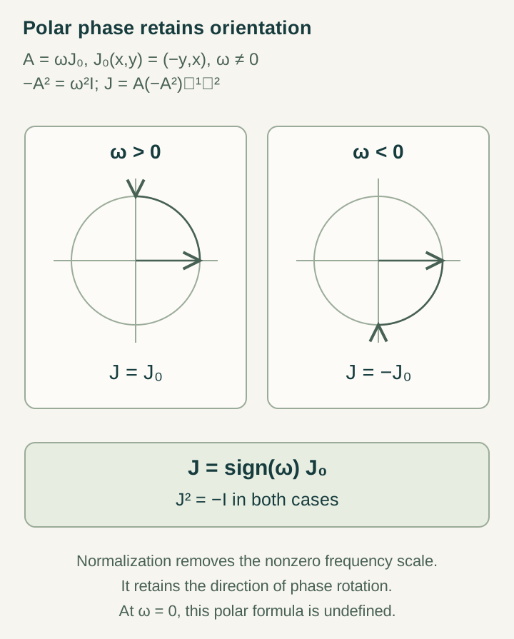
On a real plane let J₀(x,y)=(−y,x). For A=ωJ₀, ω≠0, the flow is cos(ωt)I+sin(ωt)J₀, the magnitude is |ω|I, and the polar phase is sign(ω)J₀. Increasing the speed leaves the phase unchanged; reversing the speed reverses it.

Now take two planes with A=diag(2J₀,−3J₀), in stated inverse-time units. Then Ω=diag(2I,3I) and J=diag(J₀,−J₀). Starting at (1,0,1,0), the state evolves to (cos2t,sin2t,cos3t,−sin3t). Its norm squared remains two, while each plane has its own angular speed. Dividing A by a single guessed frequency could not normalize both planes into a complex structure.

The Schrödinger convention must also be explicit. For ψ̇=JΩψ, identifying ordinary multiplication by i with J gives i aψ̇=−aΩψ. Thus that convention has Hamiltonian −aΩ. To write the same forward flow with a positive Hamiltonian H=aΩ, a>0, choose the imaginary-unit operator I_q=−J.

Both conventions are mathematically consistent when used throughout. Combining i=J, forward exp(tA) and H=+aΩ is not. The action scale a converts angular frequency to energy; the polar calculation does not set its value or identify it with a measured Planck constant. This normalization issue parallels the distinction between structural quantities and calibrated responses in the coupling chapter.

6. Separate zero modes from a gap at zero

If A has a kernel, Ω⁻¹ does not exist on the whole carrier. The orthogonal decomposition V=ker A⊕(ker A)^⊥ separates a stationary sector and a dynamic sector. The latter is invariant and supports the preceding construction. Extending J by zero on the kernel gives a partial phase whose square is minus the projector onto the dynamic sector, not minus the identity on all of V.

A stationary real line cannot carry a complex structure: a real one-by-one matrix cannot square to −1. A stationary plane can carry ±J₀, but the zero flow selects neither. In finite dimension, any globally complex carrier must have even dimension; evenness alone still does not guarantee compatibility with a specified symmetry representation.

Having no zero eigenvector is different from having frequencies bounded away from zero. For an explicit infinite-dimensional example, take the square-summable direct sum of real planes and A=⊕_n≥1(1/n)J₀. This bounded skew operator has no kernel, but its frequencies accumulate at zero. Ω=⊕(1/n)I has an unbounded inverse, while J=⊕J₀ is bounded with norm one and satisfies A=JΩ everywhere.

The example explains why an infinite-dimensional theorem uses polar decomposition or spectral calculus rather than pretending Ω⁻¹ is bounded. For unbounded generators, the factorization must hold on the common domain of A and |A|, with J preserving that domain. A positive gap is not necessary for existence of the phase, although it matters for robustness of inference from noisy data.

7. Understand what symmetry alone leaves undetermined

For a trivial action on ℝ³, every real matrix is in the commutant, but none squares to −I. Taking determinants would give (det J)²=det(−I)=−1, which is impossible over the reals. A large commutant can therefore have an empty phase space. On a trivial real plane, the orthogonal complex structures are the two quarter-turn orientations.

Multiplicity creates a different freedom. On two identical rotating planes, A=ω diag(J₀,J₀) with ω>0. Both J₊=diag(J₀,J₀) and J_mix=diag(J₀,−J₀) commute with A, preserve the norm and square to −I. However only J₊ satisfies A=J|A|. The mixed choice makes one block’s energy sign opposite if the same scalar and forward-time conventions are retained.

There are continuous families as well. Write J₊ as the common complex structure and choose an orthogonal projector P commuting with it. Then J_P=J₊(2P−I) squares to −I and is skew-adjoint. Rotating a complex one-dimensional range of P inside two complex dimensions changes J_P continuously. These choices reflect multiplicity-space freedom rather than additional observable time coordinates.

The practical lesson is to compute the actual commutant before asserting uniqueness. Independent symmetry sectors, repeated equivalent modes and stationary degrees of freedom can all preserve choices not fixed by a verbal “positive time” principle. Polar selection resolves the orientation of a specified dynamic generator; selecting that generator, its relevant sector and the treatment of residual modes remains part of the source theory.

8. Time reversal, sampling and stability

On the dynamic sector, let R be orthogonal with RAR⁻¹=−A. Then RΩR⁻¹=Ω and RJR⁻¹=−J. For either associated complex convention, R(iv)=−iR(v). A real-linear norm-preserving reversal therefore becomes antiunitary in the reconstructed complex description. On one plane, R(x,y)=(x,−y) verifies the relation directly. This is a transformation law for the supplied representation, not a derivation of every physical time-reversal quantum number.

A discrete completed record also need not reveal the continuous generator uniquely. Sampling a plane every Δ gives U(Δ)=exp(ΔωJ₀). Frequencies ω+2πk/Δ, k∈ℤ, produce exactly the same sampled matrix. Some candidate frequencies even have opposite signs. A sampling bandwidth, finer access or another phase-unwrapping rule is therefore required before the source’s oriented generator can be inferred from a single periodic update.

The no-gap example exposes a further limitation. Reverse the n-th block from +(1/n)J₀ to −(1/n)J₀ while leaving all others unchanged. The generator perturbation has norm 2/n, tending to zero, but the selected J changes by norm two on that block. Existence of polar phase is exact without a gap; uniform noise-stable phase selection near zero is a stronger demand. A physical model should state which low-frequency modes are resolved and which are retained as uncertain or stationary data.

9. Ordinary and split-complex structures do different jobs

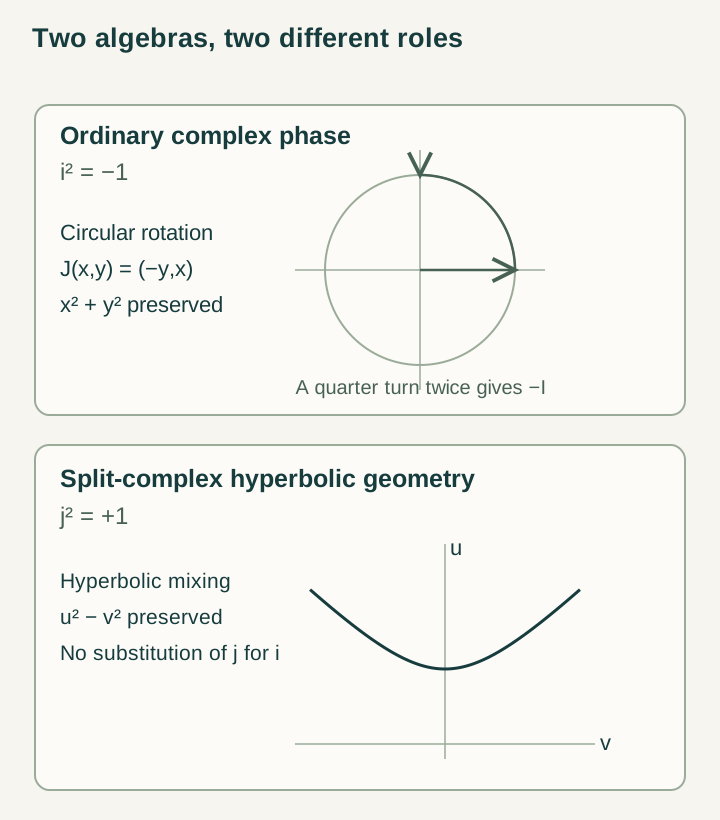
An ordinary complex unit satisfies i²=−1 and generates circular rotations. A split-complex unit j satisfies j²=+1 and generates hyperbolic mixing. For z=u+jv, the split-conjugate product is u²−v². The exponential exp(jη)=coshη+j sinhη preserves this indefinite form when acting by multiplication.

These relations cannot be exchanged by calling both quantities “complex time.” On a real plane, a circular generator J has J²=−I and is skew for a positive inner product. A hyperbolic swap K(u,v)=(v,u) has K²=I and preserves a different indefinite structure through its exponential. It is not an orthogonal imaginary unit for the original positive norm.

DTT can use these structures for distinct interfaces: circular phase in a coherent Hilbert carrier, hyperbolic algebra in a proposed temporal pairing or cone description. Connecting them requires explicit maps and compatible observables. The existence of one does not prove the other, nor does it identify two algebraic coordinates with two material clocks.

10. Derive the balancing relation for composite systems

Suppose V₁ and V₂ carry ordinary complex structures I₁ and I₂, chosen with consistent scalar conventions. The raw real tensor product has two separate phase actions, I₁⊗1 and 1⊗I₂. In a complex tensor product, moving the scalar i from one factor to the other must give the same tensor. Therefore impose the balancing relation below and complete with the compatible Hilbert tensor-product norm.

For two complex lines, choose real bases (e,I₁e) and (f,I₂f). The raw real tensor has four basis elements. Balancing identifies I₁e⊗f with e⊗I₂f, and applying the relation again gives I₁e⊗I₂f=−e⊗f. Only two real basis elements remain, exactly one complex line. More generally, complex dimensions m and n yield raw real dimension 4mn and balanced real dimension 2mn.

This reduction is a composition rule, not an automatic consequence of knowing I₁ and I₂ separately. A common source must justify why its joint preparations and operations respect that rule. Once it is supplied, familiar entanglement can be analyzed: the state (|00⟩+|11⟩)/√2 has reduced density matrix I/2 on either factor and cannot be represented by a product of two pure vectors.

The source’s unity does not remove the need to define subsystems or their accessible local operations. Entanglement depends on that operational factorization. The composition guide develops the finite examples and explains why unconditional local operations do not provide controllable signalling merely from joint coherence.

11. Connect phase to completed records without assuming the answer

A selected complex Hilbert structure supports a quantum description only after its states, observables and probability rule are specified. Under standard density-operator and Born-rule assumptions, a measurement instrument has completely positive outcome maps 𝓘_r whose sum preserves trace. For input ρ, the outcome probability is Tr 𝓘_r(ρ), and the normalized conditional state is 𝓘_r(ρ)/p_r. These are additional hypotheses of the model.

A simple completion example uses Kraus operators K_yes=√p V and K_no=√(1−p)I, with V unitary and 0<p≤1. Their squared products sum to I. The successful map is pVρV*, so its success probability p is independent of the unknown input, including when that input is entangled with a reference. This illustrates a useful completion property; the phase theorem alone does not select these Kraus operators or their success rate.

Phase sensitivity can be tested independently. Prepare ψ=(|0⟩+e^iφ|1⟩)/√2 and apply a Hadamard operation. The probability of outcome zero is |(1+e^iφ)/2|²=(1+cosφ)/2. If a prior registration dephases in the computational basis, the same later test gives 1/2. The difference records lost coherence under an explicitly chosen instrument.

A substantive SMM/DTT model should calculate which internal dynamics produces that registration, how much work and delay it costs, and how long the resulting label remains readable. Predicting only the conditional successful branch ignores incomplete attempts. A full comparison reports acceptance, failure, disturbance and retention together. The measurement and completion guide separates these operational obligations.

12. Published anchors and the next source-level tests

The published Completion principles, real commutants, and positive-frequency geometry for orthogonal Hilbert representations, DOI 10.30538/oms2026.0328, organizes the Real-commutant and polar-selection results with completion and downstream geometric modules. Its hypotheses remain essential. The Physics Letters A article, Real-commutant phase selection from real Hilbert representations, DOI 10.1016/j.physleta.2026.132085, focuses on compatible complex kinematics, residual zero-mode data and the separate composite-system requirement. Neither publication should be cited as deriving all quantum foundations or all four proposed principles without additional assumptions.

The worked calculations here extend the site’s finite polar derivation and phase guide. They provide a reproducible testing sequence: specify the real carrier and symmetry; compute the commutant; select and orient A; separate its kernel; verify J²=−I and [J,A]=0 on the dynamic sector; test sampling ambiguity and small-frequency sensitivity; then construct an independently justified composition and completion rule.

The strongest next result would remove a shared freedom across those steps. For example, one autonomous source law might select both an oriented generator and a record instrument, thereby predicting a relation between relative phase and completion delay. Such a relation must survive changes of coordinates and be compared with a model whose instrument is independently adjustable. A circular phase by itself does not establish an entropy arrow, spatial dimensionality, an absolute action scale or an electromagnetic coupling.

Continue with three-dimensional readout for the distinct quaternionic and spinor geometry, the structural count 137 for selected receiver spaces, and hydrogen for what a calibrated matter Hamiltonian adds. These connections are productive precisely because each has enough mathematical content to reveal where additional physical input is still needed.