
For invertible real skew A, J=A(−A²)⁻¹ᐟ² is orthogonal and squares to −I. Positive-energy Schrödinger form for exp(tA) uses complex multiplication i=−J when H=a(−A²)¹ᐟ².
Inputs and the object to be constructed
Let V be a finite-dimensional real inner-product space and A a real linear operator satisfying Aᵀ=−A. Consider the oriented flow U(t)=exp(tA). Initially assume A is invertible. The goal is to construct J with J²=−I and JᵀJ=I, so that real scalar multiplication can be extended to ordinary complex multiplication.
This is a conditional reconstruction from a given dynamics. The real inner product, generator and time orientation are inputs. In SMM/DTT, such a flow can represent coherent inner activity, while completed observations require an additional interface. Its vector coordinates are not the six nested temporal roles, and the ordinary complex structure is not the split-complex unit used in a hyperbolic temporal description.
Step 1: prove orthogonality and define the magnitude
Differentiate U(t)ᵀU(t). Since U̇=AU, the derivative is Uᵀ(Aᵀ+A)U=0. At t=0 the product is I, so the flow preserves the real norm for every t.
Next compute −A²=AᵀA. For nonzero v, its quadratic form is ⟨v,−A²v⟩=‖Av‖²>0 because A is invertible. Thus −A² is positive definite and has a unique positive square root Ω. It commutes with A: the two operators preserve the real invariant rotation blocks, or equivalently Ω is a spectral function of −A², which already commutes with A.
Ω measures the magnitude of the rotation rates. Its positivity supplies the specific polar normalization used in the next step.
Step 2: verify every complex-structure identity
Set J=AΩ⁻¹. Using commutation, square it: J²=A²Ω⁻²=−I. Transposing gives Jᵀ=Ω⁻¹Aᵀ=−Ω⁻¹A=−J. Therefore JᵀJ=−J²=I. The factorization A=JΩ follows immediately.
Define (r+is)v=rv+sJv. Multiplying two such scalar actions and using J²=−I reproduces the usual complex multiplication rule. Compatibility with the real norm gives a complex Hilbert-space interpretation. With the convention that the inner product is linear in its second argument, h(x,y)=⟨x,y⟩+i⟨Jx,y⟩ has the required complex linearity and h(x,x)=‖x‖².
The polar factor is unique for the supplied invertible A because Ω is uniquely positive. Other complex structures may exist on V, but they need not be the polar orientation of this flow.
Step 3: calculate a two-frequency example
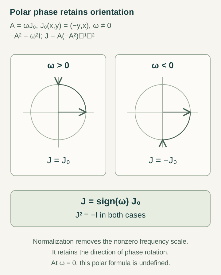
On a real plane let J0(x,y)=(−y,x). For A=ωJ0 with ω≠0, −A²=ω²I, so Ω=|ω|I and J=sgn(ω)J0. Polar normalization removes speed while retaining orientation.
On four real dimensions take A=diag(2J0,−3J0) in chosen inverse-time units. Then Ω=diag(2I,3I) and J=diag(J0,−J0). The two planes rotate at different rates and in opposite orientations, yet J²=−I on the whole space. This explicitly shows why replacing Ω by a single guessed frequency would lose information.
Open the full-size diagram →
A discrete sample of either flow does not uniquely determine A: extra full turns between samples can produce the same update matrix. Inferring a generator from discrete source records therefore requires a frequency range or another unwrapping rule.
Step 4: fix the Schrödinger sign explicitly
The real evolution satisfies ψ̇=Aψ=JΩψ. If the chosen complex imaginary unit acts as i=J, then i aψ̇=−aΩψ. In that convention the Hamiltonian is H=−aΩ. It is inconsistent to keep i=J, the same forward flow and simultaneously call H=+aΩ.
For the conventional positive Hamiltonian choose instead complex multiplication i=−J, with a>0 an action scale. Then:
H=aΩ≥0, exp(−itH/a)=exp(tJΩ)=U(t)
This is a convention and orientation choice made transparently. The finite theorem does not determine the value of a or derive a thermodynamic arrow. Changing the time orientation, complex convention or energy-sign convention must be propagated consistently through the equations.
Step 5: handle stationary modes rather than invert them
If A has a kernel, −A² is only nonnegative and Ω⁻¹ is undefined there. The orthogonal complement of ker A is invariant and the preceding construction applies on that dynamic sector. On the kernel, the flow is stationary and supplies no phase orientation.
A one-dimensional real kernel cannot support any J with J²=−I: a real scalar cannot square to −1. A two-dimensional kernel can support a quarter-turn, but choosing it is additional data. More generally, a real space carrying a complex structure must have even dimension. Appending a stationary sector therefore tests whether a claimed globally selected phase has silently supplied information absent from its dynamics.
Infinite-dimensional versions require operator domains and a careful polar construction. A finite inverse formula should not be copied onto zero-frequency or unbounded sectors without that analysis.
Step 6: track symmetry and time reversal
If a real symmetry R commutes with A, it commutes with −A², Ω and J. The selected phase therefore lies in the commutant of those source symmetries. This is the operational benefit of deriving J from the generator rather than assigning an unrelated scalar convention.
For an orthogonal reversal K satisfying KAK⁻¹=−A, the magnitude is unchanged while KJK⁻¹=−J. After choosing either associated complex convention, K conjugates the imaginary scalar and is antilinear. On one plane K(x,y)=(x,−y) demonstrates this directly. Norm preservation then makes it antiunitary in the reconstructed complex description. The statement concerns this operation on this carrier, not the transformation law of every particle species.
Result and the completion problem
The calculation supplies a unique polar phase on the nonstationary part of a specified oriented real flow, with an explicit positive-energy Schrödinger convention. It separates rates, orientation, stationary freedom and physical action normalization.
To build a quantum SMM/DTT model, the same source must also determine admissible observables, subsystem composition, states and a completion instrument. A phase-bearing carrier alone does not select Born probabilities or explain which coherence survives into public records. The phase and composition problem states that next target. The present proof provides a well-defined input to it without conflating J²=−I with the distinct split-complex relation j²=+1.
Continue with the articles
- Selecting phase by polar decomposition
Explain how a positive-time generator can select a compatible complex structure on the dynamic sector. Make clear why zero-frequency modes need separate treatment.
- Completion, commutants, and positive frequency
A reading guide to the published paper’s relationship between completion principles, real representations, and positive-frequency geometry. Focus on the theorem assumptions before discussing physical interpretations.
- Real-commutant phase selection: a paper guide
Introduce the paper’s phase-selection question in real Hilbert representations. Prepare an accessible route from the commutant to compatible complex structures and their physical interpretation.