Worked derivation: refinement dimension and the clock ratio

Define the records, scale and metric independently

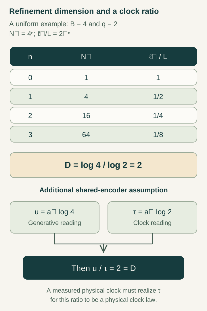
Let B≥2 be an integer, q>1 and L>0. Each completed record has exactly B distinguishable children, and each refinement reduces a comparison scale by q. A level-n address is a word of length n over an alphabet with B letters. There are N_n=Bⁿ such words, with scale ℓ_n=Lq⁻ⁿ.

For a limiting geometry use infinite words. If two words first differ after a common prefix of length m, define their distance as Lq^−m; identical words have distance zero. Two words each sharing a long prefix with a third also share at least the shorter prefix with each other. Consequently d(x,z)≤max{d(x,y),d(y,z)}, the ultrametric inequality. The distance has now been defined without using a clock.

Step 1: eliminate refinement depth

Taking logarithms gives log N_n=n log B and log(L/ℓ_n)=n log q. Eliminating n yields:

This proves a counting exponent. To identify it as a geometric dimension, the following steps compare actual covers and a normalized measure in the declared ultrametric. A finite address archive by itself is a finite metric space with Hausdorff dimension zero; the positive exponent belongs to the specified refinement limit or to a declared scaling window.

The distinction fits DTT: nested inner work creates finer distinctions, while completion makes each finite archive available. The number of internal roles is not the exponent. Several different generative architectures can implement the same count-to-scale law.

Step 2: prove the dimension upper bound

A level-n cylinder contains all infinite words with one fixed prefix of length n. It has diameter ℓ_n, and the Bⁿ cylinders cover the whole address space. For any exponent s>D, the sum of their diameter powers is:

The limit follows because B=q^D, so Bq^−s<1. These covers become arbitrarily fine as n increases. They therefore show that the Hausdorff dimension is at most D. The proof uses the supplied separation encoded by the ultrametric; overlapping geometric pictures with the same formal branching counts would require a new covering analysis.

Step 3: normalize a measure and prove the lower bound

Choose each address letter independently with probability 1/B. Every level-n cylinder then has probability B⁻ⁿ, and the probabilities of its B children sum to its probability. This defines a normalized probability measure μ on infinite addresses.

A closed ball of radius ℓ_n is exactly a level-n cylinder, so μ(ball)=(ℓ_n/L)^D. For an arbitrary radius r, choose ℓ_n≤r<qℓ_n. Then μ(ball)≤(r/L)^D. A set lies in a ball of radius equal to its diameter, giving the same upper bound for its mass.

Here the E_i form a cover with diameters at most δ and s<D. Rearranging and sending δ to zero makes the s-dimensional covering cost diverge. Thus the dimension is at least D, completing the proof.

Step 4: compare dimensions without confusing their meanings

For B=8 and q=2, D=3. At depth four, N₄=4096 and ℓ₄=L/16, with 4096=16³. For B=4 and the same q, D=2. For B=6, D=log₂6. All are exact address-space dimensions.

The B=8 example is still an ultrametric address space, not a proof of a connected three-dimensional spatial manifold. Its cylinders are separated branches, and its topology differs from ordinary continuum space. Linear detector rank, graph volume growth, spectral dimension and this address dimension can disagree. SMM/DTT needs maps and stability conditions connecting those separate measurements before interpreting their shared numerical value as one physical spatial dimension.

Step 5: derive the common logarithmic activity

Let z/z₀ be a positive dimensionless displacement ratio and Q=log(z/z₀). Suppose Q and a circular phase θ have conjugate momenta K and J. Take a work function W independent of those momenta and the single-charge Hamiltonian H=F(C), with C=K+ηJ+W. Hamilton’s equations give Q̇=F′(C) and θ̇=ηF′(C), hence Δθ=ηΔQ.

Supply independently validated contacts ending at ratios B and q. If both use one phase-to-activity calibration β, their activities are u=βη log B and τ=βη log q. With a_*=βη>0:

The endpoint laws and common calibration carry the physical content. The conserved relation alone does not prove the contacts, a monotone quantum traversal or a material clock reading.

Step 6: state which clock measures the ratio

Suppose a protected material clock is insensitive to branch activity and reads T=τ. A matter band evolving as exp(−iuH_m/a) can then be written exp(−iTDH_m/a). A coefficient v_g measured per unit u converts to Dv_g per unit T, with the Hamiltonian and physical calibration held fixed.

An equally explicit alternative clock reads T_A=u+τ. Its conversion is D/(D+1), so the same D=3 archive gives three for the protected clock and 3/4 for the alternative. No single unit conversion makes those laws agree for every D. The source must select or account for the clock response before treating the ratio as universal.

A band velocity also need not equal a sharp causal-cone slope. Identifying c=v_gD requires a separate common propagation result.

Result, verification and remaining obligations

The dimension proof and logarithmic ratio are exact under their declared inputs. The physically strongest test varies B and q while preserving the source interaction, clock mechanism and matter calibration. Count children, measure contraction and read the clock independently; do not infer one quantity from the desired equality.

Finite contact widths, imperfect completion and phase uncertainty must enter an error bound. A source realization should retain the six nested dependencies and seventh completion interface without silently making extra serial work instantaneous. The joint-source problem asks whether those same physical rules can force geometry, clocks and transport to agree, rather than merely demonstrate their compatibility.

Continue with the articles

• Why one clock model does not prove universality

  Use the ungated-clock countermodel to show that a realizable clock law need not be physically universal. Explain the extra selection principle required for all material clocks to agree.

• A quantum source for generation and completion

  Introduce the positive phase–dilation model as an explicit realization within quantum mechanics. Explain how it distinguishes inner work from completed observation without deriving quantum kinematics itself.

• From record refinement to a joint clock–band relation

  Introduce the conditional relation connecting geometry, clock response, and matter transport. Explain why the interfaces and coefficients must be independently calibrated.

• Six inner stages and one publication interface

  Explain the hierarchy of readout ranks 1, 1, 2, 2, 3, 3 followed by completion. These are nested functional roles rather than six independently readable temporal coordinates.

• Limiting speed as update scale times projection rate

  Introduce the draft’s relation between a spatial update scale, a projection rate, and the observed limiting speed. Explain why this relation alone does not fix a numerical value in laboratory units.

• A random clock behind dimensional flow

  Introduce the stochastic-renewal model in which observed time counts irregular inner events. Explain how temporal intermittency changes a diffusion probe without changing the underlying spatial manifold.

• Spectral dimension from return probabilities

  Explain how diffusion return probabilities define a scale-dependent spectral dimension. In the draft’s specified regime, temporal scaling changes that diagnostic without directly counting spatial coordinates.