
Three independent binary differences have weights 1,2,1, producing a normalized product measure on 27 sites. Exact counting, moments and entropy expose what completion retains or discards.
Inputs and the sampling convention
Take six bits d1,…,d6, each zero or one. Their address is n=Σ2a−1da, ranging from zero to 63. Group them into three pairs and define yb=d2b−1−d2b. The spatial readout is Q=ℓΣybeb, using an independent frame and positive ℓ.
Assume one complete counter sweep visits every address once and choose an address uniformly from that sweep. This supplies a definite probability measure: each six-bit string has probability 1/64. The following probabilities refer to that sampling rule. A coherent amplitude preparation or a selected completion outcome can produce another measure and requires its own instrument.
The six bits are nested counter state, not six independent laboratory clocks. Their pairing follows the architecture proved in the rank derivation.
Step 1: enumerate one pair exactly
The four input pairs are (0,0), (1,0), (0,1) and (1,1). Their differences are respectively zero, plus one, minus one and zero. Therefore the coordinate values −1,0,+1 have multiplicities 1,2,1.
Pr(Y=−1)=1/4, Pr(Y=0)=1/2, Pr(Y=+1)=1/4
The probabilities sum to one because the multiplicities sum to four. The zero value does not represent an absence of source states; it collects two different states. One has both channels inactive, while the other has both active with canceling output. A detector that reads only their difference identifies them at this instant.
Step 2: form the full product measure
Under uniform six-bit sampling the three pairs are independent. Every coordinate triple y∈{−1,0,1}³ occurs, giving 3³=27 sites. Its address multiplicity is the product of the one-pair multiplicities.
Pr(Q=ℓΣybeb)=M(y)/64
Normalization follows without listing 64 addresses: ΣyM(y)=[1+2+1]³=64. The central site has M(0,0,0)=8 and probability 1/8. A corner has no zero coordinate, so its multiplicity is one and probability 1/64. Regular spacing of sites has not produced a uniform site measure.
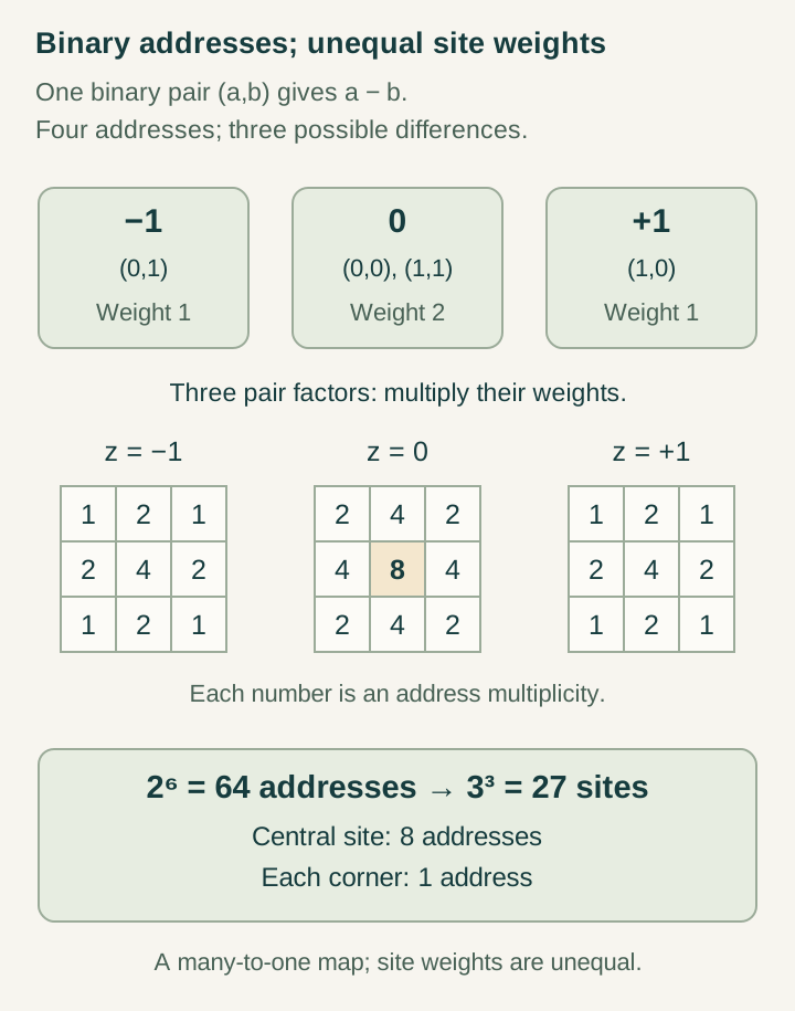
Open the full-size diagram →
A generating polynomial provides another exact check. For one pair, (1+t)(1+t⁻¹)=t⁻¹+2+t; its coefficients are the multiplicities. For three pairs use one variable per coordinate and multiply the three polynomials. The coefficient of t1y₁t2y₂t3y₃ is M(y). Setting all variables to one recovers 64.
Dividing by four and setting t=exp(ik) gives the one-coordinate characteristic function cos²(k/2). The three-coordinate characteristic function is the product of these factors. Its value at zero verifies probability normalization, and its second derivative gives the variance computed below. This is a Fourier transform of a classical probability distribution; it is not a claim that the counter prepared a quantum amplitude with that phase law.
Step 3: group the sites by nonzero coordinates
Let j be the number of nonzero coordinates. Choose those coordinates in binom(3,j) ways and choose their signs in 2j ways. Each resulting site has 3−j zero coordinates and therefore multiplicity 23−j. The total address count in that group is 8 binom(3,j).
| j | Sites | Multiplicity per site | Total probability |
|---|---|---|---|
| 0 | 1 | 8 | 1/8 |
| 1 | 6 | 4 | 3/8 |
| 2 | 12 | 2 | 3/8 |
| 3 | 8 | 1 | 1/8 |
The site counts sum to 27 and the weighted address counts to 64. With an orthonormal frame, the squared distance is jℓ². This grouping therefore also gives the complete radial distribution for that chosen metric.
Step 4: calculate moments and the radix-q extension
Symmetry gives E[Y]=0. The second moment is E[Y²]=1/4+1/4=1/2. Independence makes mixed moments vanish, so the covariance matrix of the three orthonormal coordinates is (ℓ²/2)I. Their mean squared radius is 3ℓ²/2. If the supplied frame is not orthonormal, its Gram matrix must enter the physical length calculation instead.
For a general radix q, a difference k between two uniform digits has q−|k| representatives, for |k|≤q−1. This follows by counting the allowed lower digit once the difference is fixed. The triangular multiplicities sum to q². Since one uniform digit has variance (q²−1)/12, the difference has variance (q²−1)/6.
Thus the binary result belongs to an exact family rather than a special numerical coincidence.
Step 5: distinguish reweighting from the source measure
A uniform site distribution would assign 1/27 to every site. To obtain it from weighted addresses, assign each address at site y the probability 1/[27M(y)]. Summing over its M(y) representatives then gives exactly 1/27, and summing over all sites gives one.
This is a different address preparation. Alternatively, one can use inverse-multiplicity weights to estimate uniform-site averages from the original sample, but that statistical correction does not change the underlying physical sampling process. A completion model must state which operation it actually performs. Discarding repeated labels from an archive changes a set representation; it does not by itself define how a later random observation samples that set.
The distinction is relevant to SMM/DTT because retained histories can carry different multiplicities even when their visible configurations coincide.
Step 6: quantify information loss and test prediction
The uniformly selected six-bit address has Shannon entropy six bits. One coordinate difference has entropy −2(1/4)log₂(1/4)−(1/2)log₂(1/2)=3/2 bits. Three independent coordinates therefore carry 9/2 bits. Since the output is a deterministic function of the address, the conditional entropy of the address given the site is 6−9/2=3/2 bits.
This average information loss is different from the number of retained directions or log₂27. The distribution on sites is nonuniform. It also has a dynamical consequence: addresses zero and three both map to the origin, while their successors one and four map to ℓe1 and ℓe2. No deterministic update based only on the current site reproduces both futures.
The same lost entropy follows by conditioning directly. A site with j nonzero coordinates has 23−j equally likely addresses, so its remaining address entropy is 3−j bits. The group probabilities above give E[j]=3/2, hence the averaged conditional entropy is again 3/2 bits.
Result and the meaning of completion
The exact output is a 27-site image, a normalized nonuniform measure, explicit moments and a quantified loss of address information. None of these statements identifies the private counter scan with physical motion. Carries can create projected jumps, while matter transport needs its own compatibility with retained adjacency.
For DTT, outer completion should specify whether the archive stores sites, visit counts, amplitudes, source memory or a sufficient combination. Resetting the counter at a completed boundary can simplify prediction, but every remaining variable that affects the next episode must be retained. A source model can now be tested against all these calculations together rather than only its final picture.
Continue with the articles
- Six inner stages and one publication interface
Explain the hierarchy of readout ranks 1, 1, 2, 2, 3, 3 followed by completion. These are nested functional roles rather than six independently readable temporal coordinates.
- What spatial readout forgets
Investigate information lost when a full generative state is reduced to spatial records. Explain why an apparently complete geometry may still be insufficient for autonomous prediction.
- Retained observations versus predictive states
Ask when retained information is sufficient to predict future outputs autonomously. Explain the completion criterion and why keeping observations need not keep every dynamically relevant distinction.