
For H=−DΔ−A/r with D,A>0, the normalized exponential of length 2D/A saturates a global lower bound E₁=−A²/(4D). Its linked observables test the supplied model without selecting the coupling by themselves.
1. Define an atom before interpreting its time
A hydrogen model must do more than combine opposite charges or assign a recurrence period. It must provide a normalized state, an interaction, a stable energy problem and a way to compare its predictions with observations. The nonrelativistic Coulomb system supplies an unusually complete benchmark: its ground state, radius distribution, momentum scale and bound spectrum follow from one operator.
Let r=|x| be the relative separation in three-dimensional Euclidean space. Take square-integrable complex wavefunctions and the quadratic energy form q[ψ]=D∫|∇ψ|²d³x−A∫|ψ|²/r d³x, with D,A>0 and ∫|ψ|²d³x=1. The operator is H=−DΔ−A/r, understood through the self-adjoint realization of this closed, lower-bounded form on H¹(ℝ³). The potential approaches zero at infinity, fixing the separated-particle threshold.
These are effective assumptions: continuum geometry, the Born probability rule, coherent kinetic dynamics and a particular attraction have been supplied. SMM/DTT asks how a common source could generate these ingredients and their coefficients. Solving their consequences is valuable because it supplies several linked targets instead of one fitted number.
The Coulomb singularity does not invalidate the energy problem. The three-dimensional Hardy inequality and Cauchy–Schwarz give ∫|ψ|²/r≤2‖ψ‖₂‖∇ψ‖₂. The attraction can therefore be bounded by an arbitrarily small positive multiple of the kinetic norm plus a finite multiple of the state norm. This establishes the form control needed to discuss a genuine ground state.
2. Find a candidate by direct substitution
Try a radial exponential ψ=N exp(−r/ℓ), with ℓ>0. Away from the origin, Δψ=ψ″+2ψ′/r=(ℓ⁻²−2/(ℓr))ψ. Acting with the Hamiltonian gives a constant term and a position-dependent term:
Choose ℓ=2D/A ⇒ E₁=−D/ℓ²=−A²/(4D).
The same choice fixes the characteristic length and energy. At the origin the shrinking-sphere flux of ∇ψ tends to zero, so the exponential introduces no delta-function source. The equation is valid in the appropriate weak sense.
Direct substitution finds an eigenstate, but it does not yet prove that some different shape cannot have lower energy. A trial-family minimum likewise gives only an upper bound on the true ground energy. The next step establishes a bound for every admissible state and shows that the exponential attains it.
3. Prove the global lower bound
Let r̂=x/r. Expand D∫|∇ψ+r̂ψ/ℓ|². The cross term is (D/ℓ)∫r̂·∇|ψ|². Integration by parts uses ∇·r̂=2/r; the origin contributes no point mass because the flux of r̂ through a small sphere tends to zero. Begin with suitable smooth functions and extend the identity to the form domain.
=D∫|∇ψ|²d³x−(2D/ℓ)∫|ψ|²/r d³x
+(D/ℓ²)‖ψ‖²
=q[ψ]+(D/ℓ²)‖ψ‖²≥0.
Every normalized state has energy at least −D/ℓ². The exponential satisfies ∇ψ=−r̂ψ/ℓ and makes the square vanish. It is therefore a ground state, not merely a plausible localized trial.
The equality condition also fixes its shape: ∇(exp(r/ℓ)ψ)=0, so exp(r/ℓ)ψ is constant almost everywhere. The scalar ground eigenspace is one-dimensional up to its constant complex amplitude. Spin or other internal multiplicity is separate state-space data.
For an arbitrary normalized exponential of length b, E(b)=D/b²−A/b. With x=b/ℓ and E*=D/ℓ², E(b)/E*=x⁻²−2x⁻¹ and E(b)/E*+1=(x⁻¹−1)². The trial curve explains the balance, while the global square identity proves there is no better shape outside that family.
4. Normalize the state and distinguish two densities
Spherical integration gives 1=4π|N|²∫₀∞r²exp(−2r/ℓ)dr. Since ∫₀∞rⁿexp(−λr)dr=n!/λⁿ for integer n≥0 and λ>0, the radial integral equals ℓ³/4. Choosing a positive overall normalization gives:
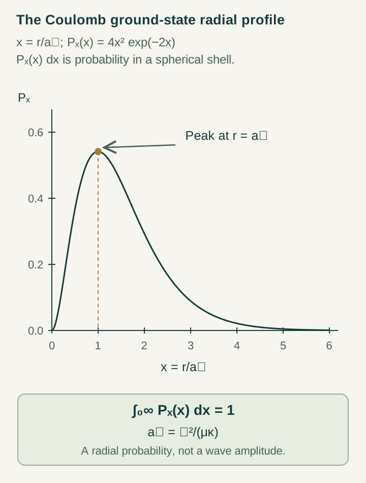
P(r)=4r²exp(−2r/ℓ)/ℓ³,
x=r/ℓ ⇒ P(r)dr=4x²exp(−2x)dx.
The density per unit volume |ψ₁|² is largest at the origin. The probability per radial interval P(r) includes the spherical-shell measure and is largest at r=ℓ. Neither statement implies a sharply defined electron orbit. A small sphere near the origin has small volume even though the local density is high.
The cumulative radial probability is also exact: Prob(r≤R)=1−exp(−2R/ℓ)[1+2R/ℓ+2(R/ℓ)²]. At R=ℓ, only 1−5exp(−2), about 0.323, of the probability lies inside the characteristic radius. A radial maximum is not a boundary containing most of the state.
This distinction is useful when evaluating a source-generated numerical profile. Compare the correct measure, check its total integral, and report whether a plotted curve is amplitude, volume density, radial probability or a cumulative distribution. Their shapes and units differ.
5. Use moments and energy balance as independent checks
The same integrals give ⟨1/r⟩=1/ℓ, ⟨r⟩=3ℓ/2 and ⟨r²⟩=3ℓ². Thus the radial variance is 3ℓ²/4. The state is localized but has a broad distribution, with standard deviation √3ℓ/2 rather than a thin orbital shell.
Because |∇ψ₁|²=|ψ₁|²/ℓ², the kinetic expectation is T=D/ℓ². The attraction has expectation V=−A/ℓ=−2D/ℓ². Their sum reproduces the eigenvalue and satisfies the Coulomb virial relation:
|E₁|ℓ=A/2.
For D=1/2 and A=1 in consistent model units, ℓ=1, E₁=−1/2, T=1/2 and V=−1. These values are exact benchmarks, not empirical measurements. A discretization should approach them together as resolution and volume errors are reduced.
Agreement with the energy alone is weak evidence for the whole state: many approximate profiles can have similar energies. Normalization, moments, kinetic balance and boundary convergence expose different errors. A source model that purports to generate hydrogen should satisfy these linked checks using one fixed scale dictionary.
6. Derive the bound-spectrum quantization
Separate variables as ψ=R(r)Yℓm, now using the angular index ℓ and writing the characteristic ground-state length as rB=2D/A to avoid ambiguity. Set u=rR. For E<0 write κ=√(−E/D). The radial equation is u″+[−κ²+A/(Dr)−ℓ(ℓ+1)/r²]u=0.
Regularity near zero suggests rℓ+1, and decay at infinity suggests exp(−κr). With x=2κr and u=xℓ+1exp(−x/2)v(x), substitution yields:
+[A/(2Dκ)−ℓ−1]v=0.
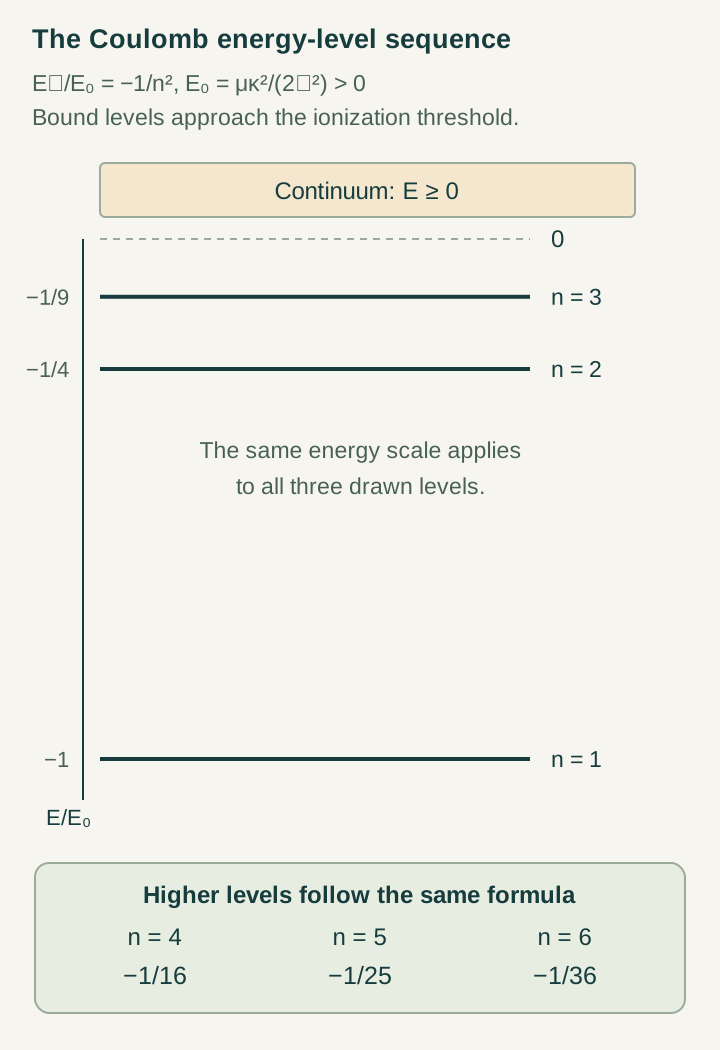
The regular confluent-hypergeometric series otherwise contains an exponentially growing contribution at large x. Normalizable bound solutions occur when the series terminates as a polynomial, requiring A/(2Dκ)−ℓ−1=nr, a nonnegative integer. Set n=nr+ℓ+1. Then κ=A/(2Dn) and:
For each n, ℓ ranges from zero to n−1 and m from −ℓ to ℓ. The scalar multiplicity is Σ(2ℓ+1)=n². This is the spinless Coulomb degeneracy. Adding a spin label is not itself a derivation of spin-orbit, magnetic or radiative effects.
The ratio of the n=2→3 excitation gap to the n=1→2 gap is (1/4−1/9)/(1−1/4)=5/27. This scale-free check tests the spectral shape while canceling the overall coefficient. Frequencies require an action–time convention, and intensities and lifetimes require coupling to radiation.
7. Introduce masses, action and the dimensionless coupling
For constituent masses m and M, use center-of-mass coordinate R=(mx₁+Mx₂)/(m+M) and relative coordinate r=x₁−x₂. Their kinetic energies separate into a free center-of-mass term and p²/(2μ), where μ=mM/(m+M). The reduced mass belongs to relative motion; it does not redefine either particle’s intrinsic mass.
Let a be the common action scale and c the matched propagation speed. Set D=a²/(2μ) and A=gac. The length and spectrum become:
En=−μc²g²/(2n²).
After quantum and electromagnetic matching, a is identified with ħ and g with α. Before that matching, these symbols describe a family of effective models. Every positive g gives a normalized Coulomb ground state. Its radius scales as g⁻¹, its binding as g², and its dimensionless radial shape is unchanged.
This scaling is a direct obstruction to deriving the coupling from binding alone. Neutrality, localization, or a stable recurrence does not select one value. The previous chapter identifies the required upstream response relation: g=scont/(4πacN), with the primitive normalization still to be derived from the source.
8. Define the speed that the ground state predicts
For the real spatial ground wavefunction, the probability current vanishes and the mean momentum vector is zero. Nevertheless, ⟨p²⟩ is positive because spatial localization requires gradients. The appropriate speed statistic is the relative root-mean-square value √⟨p²⟩/μ.
The virial relation gives ⟨p²⟩/(2μ)=−En, so vrel,rms/c=g/n. For an electron and nucleus in their center-of-mass frame, the individual momenta are p and −p, giving a different electron statistic:
ve,rms/c=(μ/me)g/n
=[M/(me+M)]g/n.
Only the infinitely heavy nucleus limit makes the electron ratio equal the relative ratio. For equal masses, each constituent’s center-of-mass RMS speed is half the relative speed. Thus the statement “α equals v/c” must identify the statistic, state and mass approximation.
As an ideal-model illustration, choose g=1/137 and M=2000me. The ground-state relative ratio is 1/137; the electron ratio is 2000/(2001×137). The binding fraction |E1|/(μc²) is 1/(2×137²). These are consequences of chosen inputs, not a measurement or independent prediction of the physical constant.
9. Distinguish persistence, preparation and corrections
With outer evolution exp(−iHT/a), an energy eigenstate changes only by a phase and retains its probability density. This gives a precise sense in which a completed atomic pattern can persist while phase evolves. It does not explain how an initially excited or unbound state reaches the ground mode. Closed unitary dynamics preserves its energy-eigenstate populations; relaxation needs additional degrees of freedom, radiation or an explicitly supplied dissipative mechanism.
The published real-commutant phase-selection work addresses how compatible complex structure can be selected from real symmetry and oriented dynamics under its hypotheses. It does not supply this Coulomb potential or determine its coefficient. Connecting the phase layer to hydrogen requires the kinetic operator, physical time and interaction to arise within one model.
Corrections must likewise be operators rather than names. For an elementary example, add δV=ε(A/rB)exp(−r/rB), with independently fixed small ε. First-order perturbation theory gives δE₁=(εA/rB)∫₀∞4x²exp(−3x)dx=8εA/(27rB). The correction is calculable because its form and coefficient were specified; fitting ε to the same measured shift would be calibration.
Realistic hydrogen additionally requires relativistic kinetics, spin, electromagnetic radiation, recoil and nuclear structure in their appropriate regimes. A source model need not solve all of them at once, but it should state its truncation and fix parameters before testing a new transition or response.
10. What would a source-level hydrogen result establish?
A substantive SMM/DTT result would derive a completed relative-state space, spatial kinetic operator and attractive response from the same nested dynamics. The source must also identify a shared action scale and physical clock, preserve the probability interpretation, and control its continuum approximation. The resulting operator should reproduce the lower bound, radial distribution, moments and spectral ratios together.
One useful intermediate study is a sequence of finite source models. Freeze the local rule and current normalization, refine the record geometry, and test convergence of multiple observables rather than refitting at each size. Separate box effects, discretization errors and physical corrections. If a common normalization fails between response and matter propagation, that failure identifies the missing bridge.
The six chapters therefore end with a connected test rather than an unconditional claim. Retained memory specifies what is predictable; readout supplies a candidate spatial sector; phase selection organizes coherent dynamics; the grammar supplies a conditional count; response supplies a coupling only after normalization; hydrogen tests the resulting dynamics through several linked observables. Each layer can strengthen the next when its additional assumptions are independently justified.
Sources and worked continuations
- Exact Coulomb ground-state derivation: domain, square completion, normalization and moments.
- Alpha and relative RMS speed; spectra and corrections; preparation and completed ground modes.
- Mohamed Haj Yousef, “Real-commutant phase selection from real Hilbert representations,” Physics Letters A 594 (2026), 132085. DOI: 10.1016/j.physleta.2026.132085. Cited for the upstream phase-selection framework, not an atomic or absolute-coupling derivation.
- Explore the normalized exponential energy family and compare it with the global proof above.