
In this article
- What an observer keeps
- An exactly soluble elimination
- A numerical benchmark
- Normalization and the vacuum question
- Three different meanings of flow
- An explicit elimination of an unobserved variable
- The strongest form of the comparison


Eliminating unobserved inner variables changes the effective law seen by a receiver. A Gaussian calculation makes this exact and connects temporal coarse graining with renormalization. The comparison also shows why nesting depth, physical elapsed time and renormalization scale cannot be identified without an additional source-derived relation.
A completed record usually retains less information than the full history that produced it. Describing only that record therefore requires a rule for eliminating or conditioning on the unobserved variables. This is one natural point of contact between DTT’s inner–outer distinction and effective theories.
Wilsonian renormalization systematically changes the effective description as degrees of freedom are integrated out and scale is adjusted. A temporal interpretation can propose that some eliminated variables belong to nested generative activity. It must still identify which variables are removed, which observables are preserved and how the resulting effective parameters are calculated. [1] [2]
Let a retained variable x and an unobserved variable y have a Gaussian weight proportional to exp[−(ax²+2bxy+dy²)/2]. Assume d > 0 and ad > b², so the quadratic form is positive definite. Completing the square in y gives d(y+bx/d)² plus (a−b²/d)x².
Integrating y therefore produces a Gaussian for x with effective coefficient aeff = a−b²/d and a normalization factor √(2π/d). The receiver’s law changes because the hidden variable was coupled to x. Discarding y without this calculation would miss the induced correction to the retained sector.
Dimensionless Gaussian variables and coefficients are used for clarity; physical units can be restored through an explicit action scale.
Choose a = 2, b = 1 and d = 2. The original determinant is three, so the Gaussian is positive definite. The retained coefficient is 2−1/2 = 3/2. Consequently the normalized variance of x is 1/(3/2) = 2/3. Omitting the coupling would have predicted variance 1/2 instead.
This difference is an observable consequence of the specified hidden coupling. It is not a new universal prediction of SMM/DTT: the coefficients were supplied. Its value is methodological. It shows how a generative variable can leave a calculable trace in outer statistics even when the variable itself is not retained as a record.
The prefactor from integrating y contributes to the partition function. It cancels from some normalized expectations but matters for quantities derived from the full free energy when its physical normalization and parameter dependence are specified. This is one reason a successful response calculation does not automatically determine an absolute gravitational vacuum energy.
In a many-mode theory, eliminated variables can induce additional operators, not just a change in one coefficient. An assumed family of simple effective laws may fail to remain closed under coarse graining. A temporal recursion must therefore justify any truncation and estimate the terms it omits. [2]
The source’s inner update order, a material clock’s elapsed time and a renormalization scale are conceptually distinct. Renormalization compares descriptions at different resolutions. Physical time describes evolution within a specified description. A change of resolution is not automatically another physical moment.
A DTT model could connect them if its generative refinement law determines both accessible scale and clock response. That relationship would be an additional constructive result, much like the joint geometry–clock relation. Merely naming a renormalization parameter inner time leaves the dynamics and calibration unchanged. [1]
The Gaussian example can be understood by completing the square. A quadratic form a x² + 2bxy + d y² equals d(y+bx/d)² + (a−b²/d)x². Integrating over y changes the normalization and leaves the effective coefficient a−b²/d for x. With a = d = 2 and b = 1, that coefficient is 3/2, and the variance under the corresponding normalized Gaussian with exponent minus one half of the form is 2/3.
The eliminated variable has not ceased to exist in the underlying two-variable model. Its effect survives in the retained coefficient. This provides a concrete interpretation of a source level whose detailed distinctions are unavailable to an outer observer but still influence completed records. Repeating such an elimination can create a hierarchy of effective descriptions. Turning that hierarchy into a renormalization group requires a defined scale transformation and rescaling rule; interpreting the scale parameter as elapsed physical time requires a separate clock construction.
A useful temporal-renormalization construction would state a source measure or quantum process, derive the reduced record law, prove consistency under successive eliminations, and identify a controlled scale regime. It would then compare physical observables across resolutions with one fixed source model.
The Gaussian example already demonstrates exact closure for a restricted family. More realistic theories add interactions, memory and nonlocal effective terms. The SMM/DTT opportunity is to derive why a particular hierarchy generates the observed effective laws and why their large-scale behavior becomes insensitive to some microscopic details. That is a concrete explanatory programme rather than a change of vocabulary.
THE SAME QUESTION, DIFFERENT STARTING POINTS
| Question | SMM/DTT | Wilsonian renormalization |
|---|---|---|
| Inner variables | Unretained generative activity may affect outer statistics. | Integrating coupled variables changes the effective action. |
| Scale | A physical source law must relate refinement to observation. | Renormalization flow compares resolutions, not necessarily elapsed time. |
| Calculation | Derive the retained law and the cost of discarded information. | The Gaussian example gives an exact Schur-complement coefficient. |
KEEP THE CONNECTION
Read a related elimination calculation for normalized response.
See why some observables miss a vacuum offset.
Compare a scale-dependent temporal probe.
Follow the common-source research sequence.
References support the comparator and the specific mathematical or interpretive claims indicated. SMM/DTT connections are developed in the analysis above.
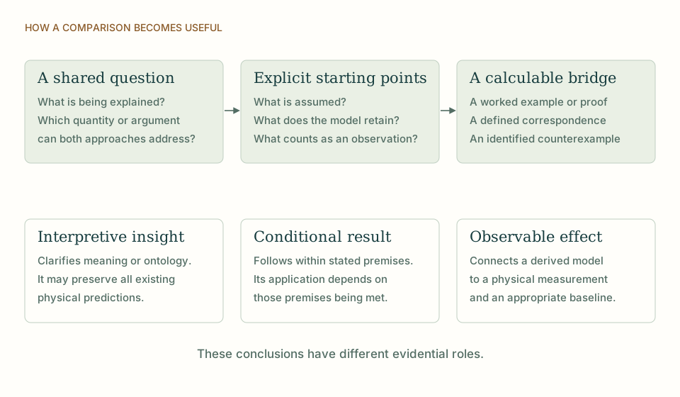
How these comparisons distinguish premises, results and physical claims