The cosmic computer: source generation and cellular automata

01A computational analogy needs physical content

A computer transforms a state according to a rule, but nearly any deterministic mathematical model can be described that way. Digital physics becomes a substantive proposal when it commits to elementary states, a physical update and resource limits. Quantum cellular automata add a particularly useful requirement: the global update is reversible while the influence of a local operation remains bounded.

SMM/DTT proposes a stronger origin story. Its source is not initially one processor located on an already existing lattice. The lattice-like relations and material records are among the outputs to be explained. A cellular automaton is therefore a benchmark for the resulting effective dynamics, while the source-to-lattice construction is an additional problem. ^[2]

02The source and its two temporal roles

The Single Monad Model begins with one nonspatial generative source. The Duality of Time Theory distinguishes the source’s inner production from the outer order in which completed records become accessible. Its six inner levels are nested functional roles of one process: a higher role organizes lower-level work. The seventh is the completion or observation interface. They are neither six independent clocks nor six additional time coordinates.

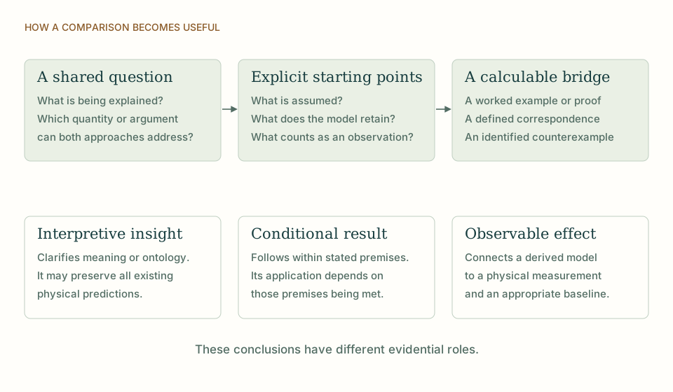
This distinction supplies a useful research question: which features of an observed world can follow from the way a source produces, retains and releases information? A concrete answer needs a state space, an autonomous update, retained memory and a rule connecting completion to an accessible measurement. In the constructions discussed here, those mathematical ingredients are stated explicitly. A successful finite example establishes what its specified mechanism can do; further arguments connect it to physical particles, spacetime or universal laws. ^[1]

03An exact local reversible example

Consider an infinite one-dimensional chain of identical finite-dimensional cells and a one-step translation that shifts every cell’s state to its right-hand neighbour. The global operation is reversible: a left shift is its inverse. An observable initially supported on one site is carried to an adjacent site after one update. After n steps its displacement is n lattice spacings.

If the spacing is a and a physical step takes Δt, the associated transport speed is a/Δt. This is an exact kinematic statement for the specified lattice automaton. It does not derive a or Δt, nor prove that all species must share that transport speed. A more general local automaton can spread support within a bounded region rather than simply translate it, but its causal radius still depends on the chosen local rule. ^[2]

04Source order is not transport order

A sequential source may visit addresses in a way that is computationally efficient but makes large jumps under a spatial readout. Such jumps do not have to be particle motion. DTT can separate the inner traversal from transport among completed records, which is one of its useful conceptual distinctions.

The physical challenge is to derive the transport rule from the same source process. If the source simply constructs a lattice and then invokes an independently chosen local automaton, it has produced a valid simulation but not explained why locality and the clock agree. The six nested functions can organize the construction, yet a different programmer could choose different neighbours or delays. A selection principle must restrict those choices before the desired geometry is imposed. ^{[2] [1]}

05Quantum resources cannot be replaced by labels

A quantum automaton evolves a noncommutative observable algebra, not merely a classical table of bit strings. Its coherent states can be entangled, and unknown quantum information cannot be freely copied. A source archive can distribute classical output labels while retaining or encoding quantum information in correlations, but those resources must be represented physically.

This matters for the cosmic-computer picture because one source executing a serial description does not automatically require less physical information than the state it simulates. A classical description of amplitudes can grow exponentially with system size. A claimed finite generative advantage should therefore specify which states and observables are represented efficiently and what error is permitted. A universal simulator is an existence result about representation; it is not by itself an explanation of why nature selects that implementation. ^{[2] [3]}

06A constructive research target

The strongest DTT version would begin with a constrained source algebra and derive an effective neighbourhood relation, a reversible local update and a calibrated clock from it. The automaton benchmark then checks the propagation cone, conservation laws and continuum behaviour. Changing a refinement parameter should not require independent retuning of all physical conversion factors.

Such a result would make the computational analogy explanatory by removing choices that an arbitrary programmer could make freely. It would also identify a possible observable restriction, such as a relation between memory capacity and transport accuracy. Until then, the analogy is still useful for building explicit examples and finding inconsistencies, provided the supplied lattice, schedule and clock are recorded as inputs rather than called derived properties of the source. ^[2]

THE SAME QUESTION, DIFFERENT STARTING POINTS

The comparison at a glance

Continue on SMONAD

• The Cosmic Computer →

  Connects this comparison with the author’s underlying construction.

• Six inner stages and one publication interface →

  Connects this comparison with the author’s underlying construction.

• Generating a neighborhood and preserving local transport →

  Connects this comparison with the author’s underlying construction.

• A finite-update cone →

  Connects this comparison with the author’s underlying construction.

• SMM/DTT research claim map: results, assumptions and open targets →

  Connects the comparison to the programme’s current statement of results and assumptions.