
Matching a curvature coefficient κ to the stated Einstein-action convention gives G=c³ℓ*²/(16πaκ). The substantive source calculation is the metric response κ and its common normalization with matter.
From spatial readout to geometric response
SMM/DTT treats spatial relations as completed results of a common generative process. A gravity programme must therefore ask how changing those relations changes the action of the process. This is a definite calculation only after the model specifies what is varied: distances, completion weights, transport rules, cell volumes or another operational metric input.
A local rank-three readout alone does not determine that response. Nor does a nested order of generation automatically select a Lorentzian metric or Einstein dynamics. The constructive route is to establish a long-distance geometry, couple the source model to a controlled geometric deformation, and calculate the effective action that survives completion.
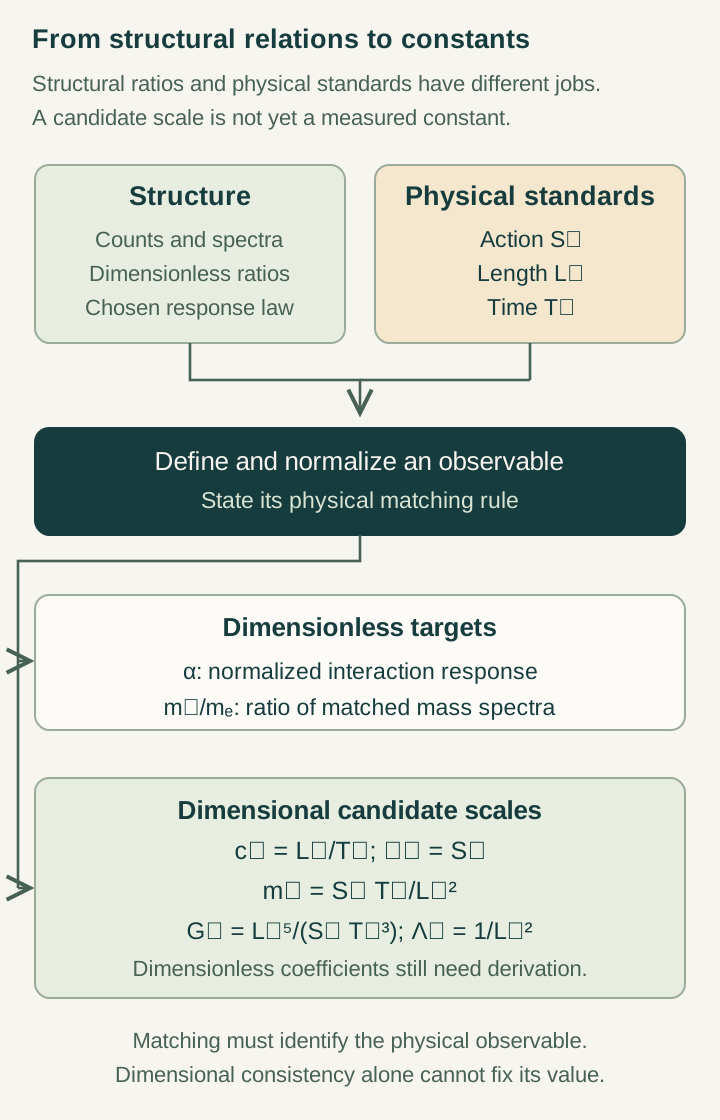
Use one dictionary for length, time and action
Let y denote dimensionless coordinates and set xμ=ℓ*yμ, using x0=ct. Let τ* convert a completed update into physical duration, and let υ be a dimensionless propagation coefficient. The common speed dictionary is c=υℓ*/τ*.
The action scale a converts the dimensionless source action into physical action. These quantities must refer to compatible measurements: the clock cannot be a controller label in one equation and a matter clock in another. A bound on propagation also needs an argument before it is identified with the sharp signal coefficient used by the gravitational and matter sectors. This is where DTT’s shared generation must become a shared operational law.
Match the curvature term step by step
Suppose a controlled effective expansion has Sgeom/a=∫d⁴y√|g|(κR̂−r+⋯), where R̂=ℓ*²R and r is the constant term. Coordinate conversion gives d⁴y=d⁴x/ℓ*⁴, so the physical curvature coefficient is aκ/ℓ*².
Using the convention SEH=[c³/(16πG)]∫d⁴x√−g(R−2Λ), equality of the curvature coefficients gives:
G = c³ℓ*²/(16πaκ)
This matching is exact under the declared continuum interpretation and action convention. It organizes the target calculation but does not calculate κ. The omitted terms and the matter coupling determine whether the full effective dynamics actually has the desired gravitational limit.
Check units and vary one coefficient
Action has dimensions ML²/T, so the right-hand side has dimensions (L/T)³L²/(ML²/T)=L³/(MT²), the dimensions of G. The check detects a missing conversion factor but cannot choose a dimensionless response coefficient.
For a simple sensitivity example, keep a, c and ℓ* fixed. Doubling κ halves G: a stiffer curvature response corresponds to a weaker coupling in this convention. Doubling ℓ* at fixed c instead multiplies G by four. If τ* is held fixed while ℓ* changes, c changes too; that is a different comparison. The gravity workbench makes these shared dependencies visible.
Remove units to expose the real target
Combine the gravitational dictionary with me=aεe/(c²τ*) and c=υℓ*/τ*. The conversion scales cancel from the dimensionless gravitational strength:
Open the full-size diagram →
Here ge denotes gravitational strength, not the electron’s magnetic g-factor. A source theory must constrain the electron gap, geometric response and propagation coefficient together to predict this quantity. For example, multiplying εe by two and κ by four leaves it unchanged at fixed υ. Matching one measured gravitational ratio therefore does not uniquely reconstruct the internal source parameters.
What computing κ actually involves
The microscopic model must specify its state, measure, regulator and geometric dependence before variation. A normalization factor independent of a phase source can still depend on the metric. Dropping it because it cancels from a phase probability may therefore discard part of the geometric response.
Once the action is defined, the calculation should isolate its curvature term and bound the remaining terms in the stated regime. Positive κ selects the intended sign of that term, but higher-derivative modes, a consistent Lorentzian continuation, conserved matter coupling and a Newtonian limit still need examination. A geometric inequality or a dimensionless stiffness can contribute to this programme only after its normalization is connected to the same physical action.
A concrete source-level objective
The next useful result is a family of explicitly generated geometries for which the completed source action can be evaluated under small deformations. Extract κ from those values without calibrating it to G, and use the same model to calculate the matter gap and propagation coefficient. The unit-free combination above then becomes a cross-sector output.
Fitting κ=c³ℓ*²/(16πaGref) is a legitimate calibration, but reproducing G afterwards is the inverse calculation. An additional geometric response, matter relation or controlled correction would supply a new test. The vacuum guide extends the same action to its constant term, where a different information problem arises.
Continue with the articles
- A dependency map for physical constants
Introduce the constants program as a chain from completion dynamics to response and then physical matching. Identify which quantities are structural, calibrated, or still free.
- Identifiability: can observations determine the model?
Explain why a collection of observable constants can leave parameter directions unresolved. Use the draft’s two remaining directions to distinguish a good fit from unique reconstruction.
- Prediction after calibration
Present the calibration-fiber criterion for a conditional prediction. An additional observable must be fixed across the allowed calibrated models to avoid merely reusing its target value.
- Why normalized response misses absolute vacuum offsets
Explain the obstruction to inferring gravitating vacuum energy from normalized completion response. Adding an invisible offset exposes information that the response alone cannot determine.
- A common dimensional dictionary
Introduce the conversion between dimensionless model outputs and quantities expressed in physical units. Explain why unit consistency is necessary but does not determine an absolute action, length, or time scale.